A model does not fail loudly. It keeps returning scores in the right range, the service stays green, and the business notices six weeks later that approval rates moved or fraud losses climbed. By then the training data that would explain it has been overwritten and the retraining cadence has already passed. Model drift monitoring exists to close that gap from weeks to hours, and the reason we build it on ClickHouse is that the monitoring is a set of aggregate queries over every prediction the model ever made, and that is precisely the workload ClickHouse is built for.
This post is the model drift monitoring we operate for customers running fraud, credit, pricing and demand models in production, written as the runbook we hand to the team that owns it: what to log on every prediction, which statistic to compute for which kind of feature, the ClickHouse queries that compute them from a prediction log that grows by hundreds of millions of rows a month, the thresholds and how they are tied to money rather than to a textbook constant, and the routing that decides whether an alert means retrain, roll back or ignore.
Everything here runs on ClickHouse 25.x or later, self-managed or Cloud. Thresholds and volumes are illustrative unless a measurement source is named.
Log the prediction, the inputs and the version, or nothing later is possible
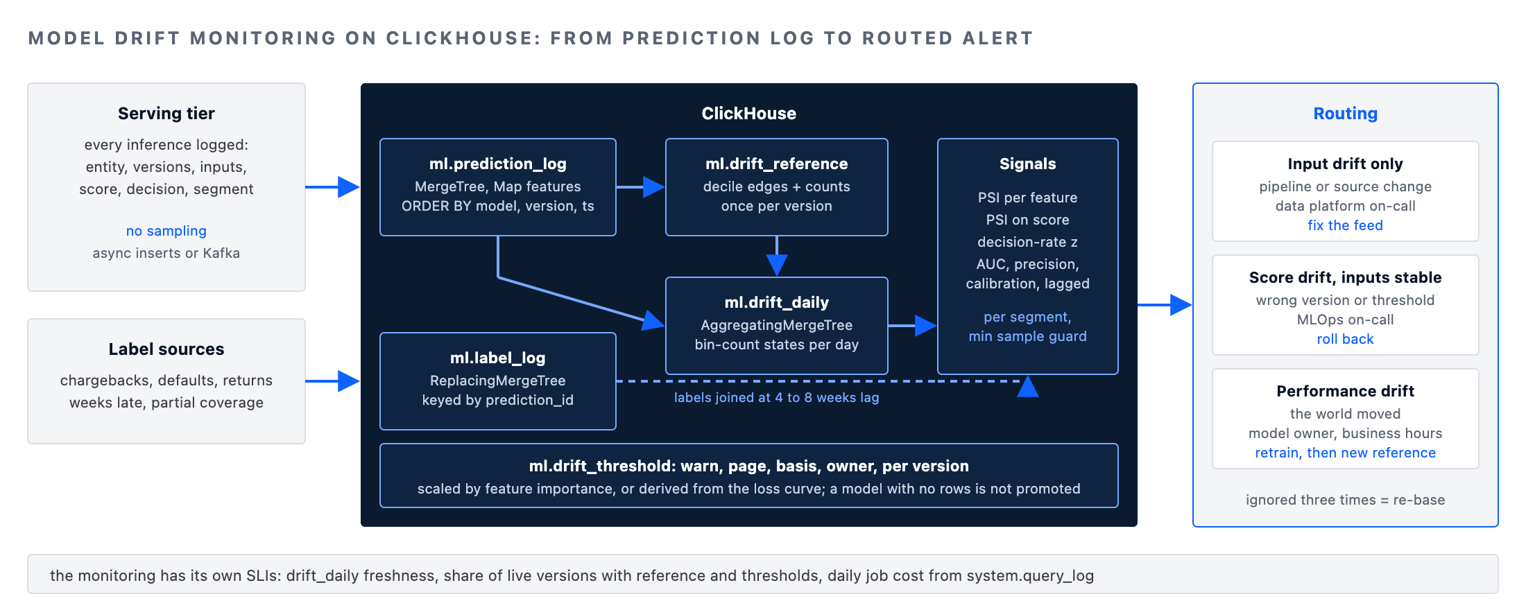
Every other part of model drift monitoring depends on a prediction log that captures, for each inference, the entity, the timestamp, the model and feature versions, the full input vector as the model saw it, and the output. Sampling is the first model drift monitoring mistake we see: a one percent sample is fine for a distribution over millions of predictions and useless when the question is what happened to one customer, or to the small segment where the drift actually lives. Log everything; the model drift monitoring storage cost on ClickHouse with a sensible sort key and compression is a rounding error next to a mis-priced quarter.
-- Prediction log: the single source for model drift monitoring (ClickHouse 25.x+)
CREATE TABLE ml.prediction_log
(
    model_name        LowCardinality(String),
    model_version     LowCardinality(String),
    feature_semver    LowCardinality(String),
    entity_id         UInt64,
    prediction_id     UUID,
    served_ts         DateTime64(3, 'UTC'),
    features_num      Map(LowCardinality(String), Float64),   -- numeric inputs
    features_cat      Map(LowCardinality(String), String),    -- categorical inputs
    score             Float64,
    decision          LowCardinality(String),                 -- approve, decline, review
    latency_ms        UInt16,
    segment           LowCardinality(String)                  -- country, channel, product
)
ENGINE = ReplicatedMergeTree(
    '/clickhouse/tables/{shard}/ml/prediction_log',
    '{replica}'
)
PARTITION BY toYYYYMM(served_ts)
ORDER BY (model_name, model_version, served_ts, entity_id)
TTL toDateTime(served_ts) + INTERVAL 24 MONTH TO VOLUME 'cold'
SETTINGS index_granularity = 8192;

-- Labels arrive later, from a different system, at a different cadence
CREATE TABLE ml.label_log
(
    model_name        LowCardinality(String),
    prediction_id     UUID,
    entity_id         UInt64,
    label_ts          DateTime64(3, 'UTC'),
    label             UInt8,                                   -- 1 = fraud confirmed, default, etc.
    label_source      LowCardinality(String)
)
ENGINE = ReplicatedReplacingMergeTree(
    '/clickhouse/tables/{shard}/ml/label_log',
    '{replica}',
    label_ts
)
PARTITION BY toYYYYMM(label_ts)
ORDER BY (model_name, prediction_id);
The Map columns are a deliberate model drift monitoring trade. A fixed column per feature is faster to scan but couples the log schema to every model's feature list; a map lets one table serve every model and every version, and ClickHouse reads only the keys a query touches. The sort key puts version before time because model drift monitoring almost always compares one version's behaviour across time or two versions across the same window, and both become range reads. The TTL moves two-year-old predictions to object storage rather than deleting them; regulated customers need the history for model-risk evidence.
Three kinds of drift, and the statistic that fits each
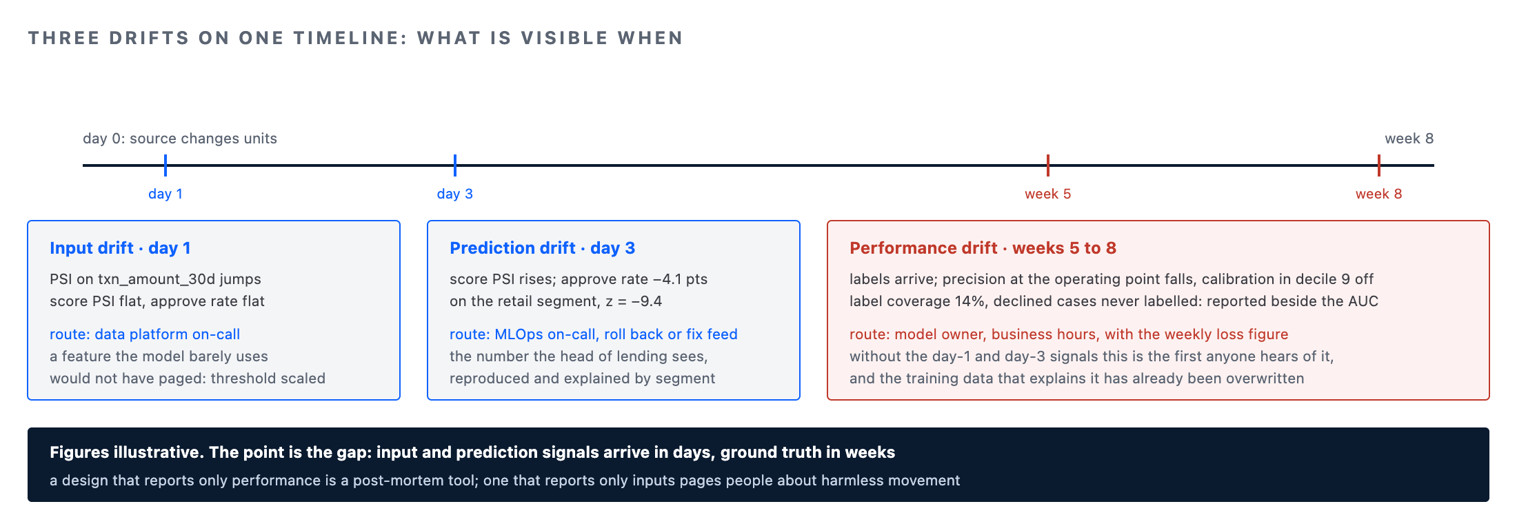
Model drift monitoring conflates three different things when it is done badly. Input drift is the distribution of a feature moving away from what the model was trained on, which is visible immediately. Prediction drift is the distribution of the model's scores moving, which is also immediate and is usually the first thing the business notices as an approval-rate change. Performance drift is the model's accuracy against ground truth degrading, which is the thing that costs money and the thing that can only be measured once labels arrive, often weeks later.
A model drift monitoring design that reports only the third is a post-mortem tool; one that reports only the first pages people about features that moved harmlessly.
| Signal | Statistic we use | Reference window | Where it fails |
|---|---|---|---|
| Numeric input drift | Population stability index over decile bins | Training set, or the first 30 days of the current version | Heavy tails: bins from quantiles, never fixed widths |
| Categorical input drift | PSI over categories, with a pooled "other" bucket | Same as numeric | New categories: a value unseen in training is its own alert |
| Prediction drift | PSI on score deciles plus decision-rate delta | Trailing 28 days of the same version | Seasonality: compare like-for-like weekday and hour |
| Performance drift | AUC, precision at the operating threshold, calibration by decile | Validation-set figures recorded at promotion | Label delay and label bias: declined cases never get a label |
| Segment drift | All of the above, per segment, compared to the overall figure | Overall population | Small segments: minimum sample size before alerting |
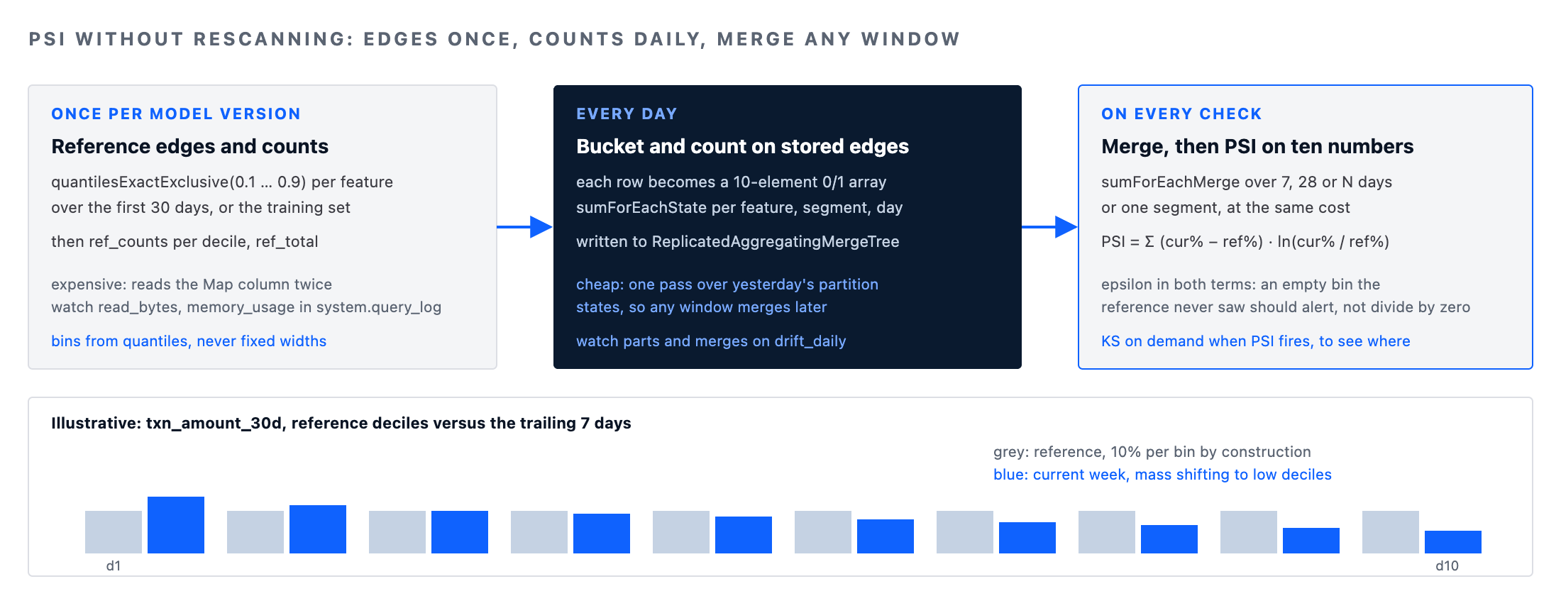
We use quantile-based PSI rather than a Kolmogorov-Smirnov statistic for daily model drift monitoring checks because PSI is additive over bins, which means it can be computed from pre-aggregated bin counts stored per day and merged over any window without touching the raw rows. KS needs the full empirical distribution and is what we run on demand when PSI fires, to see where in the distribution the movement is.
Bins from the reference, counts from the day, PSI from the merge
The core model drift monitoring query has three parts, and separating them is what keeps it cheap. The bin edges come from the reference window once, as the deciles of each feature, and are stored. Each day's predictions are bucketed against those stored edges and counted per bin, and the counts land in an aggregating table. PSI is then a small query over two sets of ten counts, and comparing any window to the reference is a merge rather than a scan.
-- Reference bin edges per feature, computed once per model version from its first 30 days
CREATE TABLE ml.drift_reference
(
    model_name        LowCardinality(String),
    model_version     LowCardinality(String),
    feature           LowCardinality(String),
    edges             Array(Float64),             -- 9 interior decile edges
    ref_counts        Array(UInt64),              -- 10 bins
    ref_total         UInt64,
    computed_at       DateTime DEFAULT now()
)
ENGINE = ReplicatedReplacingMergeTree(
    '/clickhouse/tables/{shard}/ml/drift_reference',
    '{replica}',
    computed_at
)
ORDER BY (model_name, model_version, feature);

INSERT INTO ml.drift_reference (model_name, model_version, feature, edges, ref_counts, ref_total)
WITH
    ref_edges AS
    (
        SELECT
            k                                                                        AS feature,
            quantilesExactExclusive(0.1, 0.2, 0.3, 0.4, 0.5, 0.6, 0.7, 0.8, 0.9)(v)  AS edges
        FROM ml.prediction_log
        ARRAY JOIN mapKeys(features_num) AS k, mapValues(features_num) AS v
        WHERE model_name = 'fraud_auth' AND model_version = '4.2.0'
          AND served_ts >= '2026-07-01' AND served_ts < '2026-07-31'
        GROUP BY k
    )
SELECT
    p.model_name,
    p.model_version,
    k                                                       AS feature,
    e.edges,
    -- bin membership per row as a 10-element 0/1 array, summed element-wise
    sumForEach(arrayMap(i -> toUInt64(
        (i = 0  AND v <  e.edges[1]) OR
        (i = 9  AND v >= e.edges[9]) OR
        (i BETWEEN 1 AND 8 AND v >= e.edges[i] AND v < e.edges[i + 1])
    ), range(10)))                                          AS ref_counts,
    count()                                                 AS ref_total
FROM ml.prediction_log AS p
ARRAY JOIN mapKeys(p.features_num) AS k, mapValues(p.features_num) AS v
JOIN ref_edges AS e ON e.feature = k
WHERE p.model_name = 'fraud_auth' AND p.model_version = '4.2.0'
  AND p.served_ts >= '2026-07-01' AND p.served_ts < '2026-07-31'
GROUP BY p.model_name, p.model_version, k, e.edges;
That query is the expensive one in model drift monitoring, and it runs once per version. On a month of 300 million predictions with forty numeric features it reads the map column twice, once for the edges and once for the counts, and aggregates per key; check system.query_log for read_bytes and memory_usage, and if memory is the constraint, run it per feature with a WHERE k = ... filter rather than raising max_memory_usage. The daily counts are cheap by comparison and are written by a scheduled job into an aggregating table.
-- Daily bin counts per feature, per segment, stored as states so any window merges
CREATE TABLE ml.drift_daily
(
    model_name        LowCardinality(String),
    model_version     LowCardinality(String),
    feature           LowCardinality(String),
    segment           LowCardinality(String),
    d                 Date,
    bin_counts        AggregateFunction(sumForEach, Array(UInt64)),
    n                 AggregateFunction(sum, UInt64)
)
ENGINE = ReplicatedAggregatingMergeTree(
    '/clickhouse/tables/{shard}/ml/drift_daily',
    '{replica}'
)
PARTITION BY toYYYYMM(d)
ORDER BY (model_name, model_version, feature, segment, d);

INSERT INTO ml.drift_daily
SELECT
    p.model_name,
    p.model_version,
    k                                                       AS feature,
    p.segment,
    toDate(p.served_ts)                                     AS d,
    sumForEachState(arrayMap(i -> toUInt64(
        (i = 0  AND v <  r.edges[1]) OR
        (i = 9  AND v >= r.edges[9]) OR
        (i BETWEEN 1 AND 8 AND v >= r.edges[i] AND v < r.edges[i + 1])
    ), range(10)))                                          AS bin_counts,
    sumState(toUInt64(1))                                   AS n
FROM ml.prediction_log AS p
ARRAY JOIN mapKeys(p.features_num) AS k, mapValues(p.features_num) AS v
JOIN ml.drift_reference AS r
  ON r.model_name = p.model_name AND r.model_version = p.model_version AND r.feature = k
WHERE p.served_ts >= yesterday() AND p.served_ts < today()
GROUP BY p.model_name, p.model_version, k, p.segment, d;

-- PSI for the trailing 7 days against the reference, per feature, overall population
WITH
    0.0005 AS eps,
    cur AS
    (
        SELECT
            feature,
            sumMerge(n)                     AS n_7d,
            sumForEachMerge(bin_counts)     AS cur_counts
        FROM ml.drift_daily
        WHERE model_name = 'fraud_auth' AND model_version = '4.2.0'
          AND d >= today() - 7
        GROUP BY feature
    )
SELECT
    c.feature,
    c.n_7d,
    arraySum(arrayMap((a, b) ->
        ((a + eps) - (b + eps)) * log((a + eps) / (b + eps)),
        arrayMap(x -> x / c.n_7d,       c.cur_counts),
        arrayMap(x -> x / r.ref_total,  r.ref_counts)))     AS psi_7d
FROM cur AS c
JOIN ml.drift_reference AS r
  ON r.model_name = 'fraud_auth' AND r.model_version = '4.2.0' AND r.feature = c.feature
ORDER BY psi_7d DESC
LIMIT 15;
Because the model drift monitoring daily table stores aggregate states, the same query with d >= today() - 28 or a segment filter costs the same and needs no re-scan of the log. The epsilon guards against empty bins; a bin the reference never saw and the current week fills is exactly the case PSI should scream about, and it will, but it should not divide by zero doing so.
Prediction drift and the number the business already watches
In model drift monitoring, score distribution drift is computed the same way with the score itself as the feature, and we add one thing the modelling team rarely thinks to add: the decision rate. An approval rate that moves from 71 percent to 66 percent week over week is what the head of lending sees on their dashboard, and if model drift monitoring cannot reproduce that number and explain it in terms of score movement and segment mix, the monitoring will not be trusted. So the decision-rate delta is computed alongside PSI on the score, by segment, against a like-for-like window of the same weekdays.
-- Decision-rate movement by segment, like-for-like weekdays, with sample-size guard
WITH
    cur AS
    (
        SELECT segment, count() AS n, countIf(decision = 'approve') / count() AS approve_rate
        FROM ml.prediction_log
        WHERE model_name = 'fraud_auth' AND model_version = '4.2.0'
          AND served_ts >= today() - 7 AND toDayOfWeek(served_ts) BETWEEN 1 AND 5
        GROUP BY segment
    ),
    ref AS
    (
        SELECT segment, count() AS n, countIf(decision = 'approve') / count() AS approve_rate
        FROM ml.prediction_log
        WHERE model_name = 'fraud_auth' AND model_version = '4.2.0'
          AND served_ts >= today() - 35 AND served_ts < today() - 7
          AND toDayOfWeek(served_ts) BETWEEN 1 AND 5
        GROUP BY segment
    )
SELECT
    c.segment,
    c.n                                             AS n_current,
    round(r.approve_rate, 4)                        AS approve_rate_ref,
    round(c.approve_rate, 4)                        AS approve_rate_now,
    round(c.approve_rate - r.approve_rate, 4)       AS delta,
    -- two-proportion z, so a 2-point move on 400 rows is not treated like one on 400,000
    round((c.approve_rate - r.approve_rate) /
          sqrt(r.approve_rate * (1 - r.approve_rate) * (1 / c.n + 1 / r.n)), 2) AS z
FROM cur AS c
JOIN ref AS r USING (segment)
WHERE c.n >= 2000
ORDER BY abs(z) DESC;
Performance drift with labels that arrive late and only for some rows
The honest part of model drift monitoring is admitting that ground truth is late and biased. A fraud label arrives when a chargeback does, weeks after the authorisation; a default label arrives months after a credit decision; and neither ever arrives for the applications the model declined. So performance is computed on a lagged window, labelled rows only, and reported with the label coverage beside it so nobody reads an AUC computed on 12 percent of predictions as if it were the whole population.
-- Performance on the predictions old enough to have labels, with coverage reported
WITH
    scored AS
    (
        SELECT p.prediction_id, p.score, p.segment, l.label
        FROM ml.prediction_log AS p
        LEFT JOIN ml.label_log FINAL AS l
          ON l.model_name = p.model_name AND l.prediction_id = p.prediction_id
        WHERE p.model_name = 'fraud_auth' AND p.model_version = '4.2.0'
          AND p.served_ts >= today() - 63 AND p.served_ts < today() - 35   -- label lag ~4 weeks
    )
SELECT
    segment,
    count()                                                         AS predictions,
    countIf(label IS NOT NULL) / count()                            AS label_coverage,
    arrayAUC(groupArrayIf(score, label IS NOT NULL),
             groupArrayIf(label, label IS NOT NULL))                AS auc_labelled,
    countIf(label = 1 AND score >= 0.80) /
        nullIf(countIf(score >= 0.80 AND label IS NOT NULL), 0)      AS precision_at_operating_pt
FROM scored
GROUP BY segment
HAVING countIf(label IS NOT NULL) >= 500
ORDER BY auc_labelled ASC;
For performance model drift monitoring, the validation-set AUC recorded at promotion is stored in the model registry with the version, and the alert compares against that figure, not against last week. Calibration by score decile, the share of decile-nine predictions that were actually fraud, is computed the same way and is usually the earlier model drift monitoring warning: a model can hold its rank ordering while its probabilities drift, and a decision threshold set on those probabilities quietly moves.
Thresholds tied to money, not to 0.2
Every model drift monitoring guide repeats the same PSI folklore: under 0.1 is stable, 0.1 to 0.25 is moderate, over 0.25 is significant. Those constants came from credit scorecards decades ago and mean nothing for a feature whose movement the model barely uses.
We set model drift monitoring thresholds two ways. For input drift, each feature's threshold is scaled by its importance in the model, so a PSI of 0.15 on the top feature alerts and the same value on a feature with near-zero gain does not. For prediction and performance drift, the threshold is derived from the loss curve: the modelling team states, at promotion, how much decision-rate or precision movement translates to a business cost the owner cares about, and that is the alert line.
-- Thresholds live in a table, per version, with the reasoning attached
CREATE TABLE ml.drift_threshold
(
    model_name        LowCardinality(String),
    model_version     LowCardinality(String),
    signal            LowCardinality(String),      -- 'psi:feature_name', 'psi:score', 'approve_rate', 'auc'
    warn              Float64,
    page              Float64,
    basis             String,                      -- 'importance 0.31 x base 0.25', 'loss curve: 2pt = $X/wk'
    owner_email       String,
    set_at            DateTime DEFAULT now()
)
ENGINE = ReplicatedReplacingMergeTree(
    '/clickhouse/tables/{shard}/ml/drift_threshold',
    '{replica}',
    set_at
)
ORDER BY (model_name, model_version, signal);

-- Illustrative: per-feature PSI thresholds scaled by feature importance from the registry
INSERT INTO ml.drift_threshold
SELECT
    'fraud_auth', '4.2.0',
    concat('psi:', feature),
    0.10 * (1 - importance) + 0.05           AS warn,     -- important features alert sooner
    0.25 * (1 - importance) + 0.10           AS page,
    concat('importance ', toString(importance), ' scaled from base 0.10 / 0.25'),
    'fraud-model-owner@example.com'
FROM ml.feature_importance
WHERE model_name = 'fraud_auth' AND model_version = '4.2.0';
The basis column is not model drift monitoring documentation for its own sake. When an alert fires at 03:00, the on-call engineer reads why this threshold exists before deciding whether to act, and when the model owner is asked six months later why a page was ignored, the reasoning that was current at the time is on the row.
Routing: what a model drift monitoring alert actually means
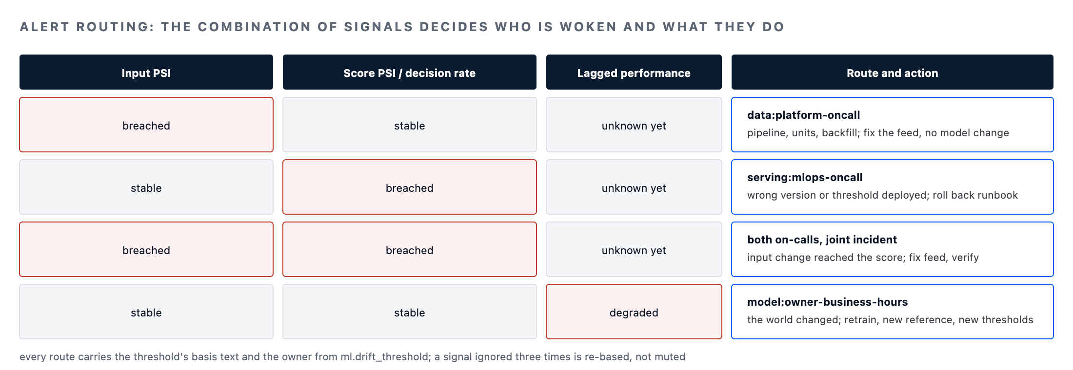
Model drift monitoring produces three kinds of action and the routing has to say which. Input drift on a feature with no prediction drift is usually a data pipeline event, a source that changed units or a feature-store backfill, and it goes to the data platform on-call with the feature name, not to the modelling team. Prediction drift without input drift is a model-serving event, a wrong version deployed or a threshold changed, and it pages the MLOps rotation with a rollback runbook.
Performance drift with stable inputs and predictions is the world changing under a model that is behaving as designed, and that is a retrain decision for the model owner, made in business hours with the loss figure in hand.
-- Alert view: every breached threshold with its routing class, evaluated by the scheduler
CREATE VIEW ml.drift_alerts AS
WITH
    psi AS
    (
        SELECT concat('psi:', feature) AS signal, psi_7d AS value
        FROM ml.drift_psi_7d                    -- materialised from the PSI query above
        WHERE model_name = 'fraud_auth' AND model_version = '4.2.0'
    )
SELECT
    t.signal,
    p.value,
    t.warn,
    t.page,
    multiIf(p.value >= t.page, 'page', p.value >= t.warn, 'warn', 'ok')      AS level,
    multiIf(
        startsWith(t.signal, 'psi:score') OR t.signal = 'approve_rate',      'serving:mlops-oncall',
        startsWith(t.signal, 'psi:'),                                        'data:platform-oncall',
        t.signal IN ('auc', 'precision', 'calibration'),                     'model:owner-business-hours',
        'unrouted')                                                          AS route,
    t.owner_email,
    t.basis
FROM ml.drift_threshold FINAL AS t
JOIN psi AS p USING (signal)
WHERE p.value >= t.warn;
Two rules keep model drift monitoring routing honest. An alert that is routed and then ignored three times in a row is a threshold that needs re-basing, and the platform reports that count per signal. And a retrain triggered by performance drift is not complete until the new version's reference bins are computed and the thresholds table has rows for it; a model with no thresholds is not monitored, and the deploy pipeline refuses to promote it.
Operating the model drift monitoring itself
The model drift monitoring platform is a production system on the same footing as the model. Its own SLIs are the freshness of drift_daily against the log, the share of active model versions with a reference and a threshold set, and the cost of the daily job from system.query_log. On ClickHouse the operational watch points are the parts count on prediction_log during high-volume hours, since a burst of small inserts from many serving replicas is the classic cause of "too many parts", which we handle with async inserts from the serving tier, and the merge backlog on drift_daily in system.merges, which grows if the daily job writes many small states.
Where the serving tier already logs to Kafka, model drift monitoring ingestion changes shape: the log table is fed by a Kafka engine table and materialised view rather than by direct inserts, and the same pattern from our feature store architecture post applies: the streaming path writes the same columns as any batch backfill, so a replayed day reconciles cleanly.
Working with MinervaDB on model drift monitoring
Model drift monitoring is part of our MLOps consulting practice, typically built in the second phase of an engagement once the prediction log and the feature registry exist, and it draws on the same ClickHouse engineering our 24×7 teams operate for real-time analytics customers. The thresholds-as-data and routing discipline here is what our decision intelligence work depends on for outcome capture, and the two are usually built together.
Under managed model drift monitoring operations the freshness, coverage and cost SLIs above are monitored by our on-call under the standard S1 to S4 response commitments, with a stale or missing drift signal on a production model treated as an S2. As always: test every table, query and threshold here against your own prediction volumes before applying it to production, and keep a tested restore posture for the prediction log; for a regulated model it is evidence, not telemetry.
Running this in production?
MinervaDB provides ClickHouse Consulting with 24x7 coverage and a 15-minute S1 response. Talk to an engineer.