A CPG demand forecasting pipeline is not a model. The model is the part that gets the conference talk; the pipeline is the part that decides whether the number a planner sees on Monday morning was built from data that existed on Monday morning, at the grain the planner actually orders in, reconciled so that the brand total equals the sum of its SKUs. When the pipeline is wrong, a better model makes the wrong number more confidently.
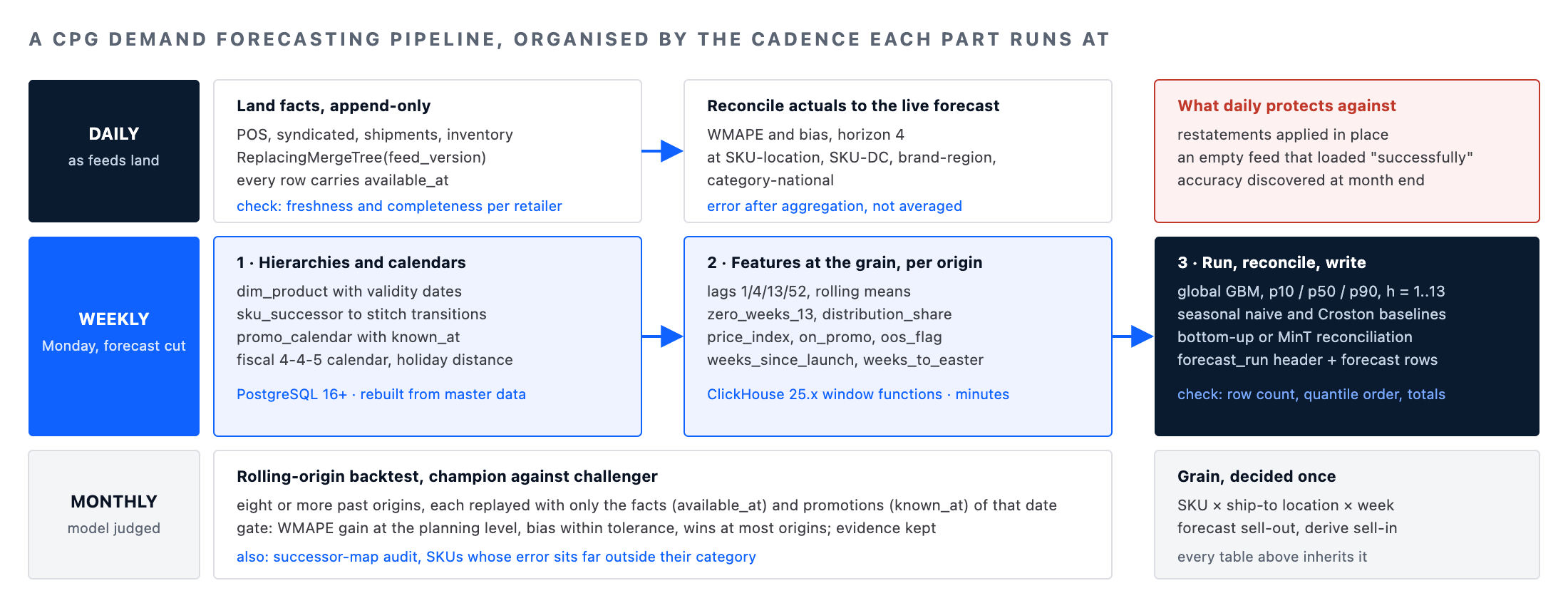
This post describes the demand forecasting pipeline we build for consumer goods manufacturers, organised the way it runs: by cadence. Some of it happens every day as retailer feeds land, some of it weekly when the forecast is cut, some of it monthly when a challenger model is judged against the champion. Each cadence has its own tables, its own SQL and its own failure modes, and separating them is what keeps a demand forecasting pipeline operable once it has two hundred million SKU-location-weeks in it.
The reference stack is ClickHouse 25.x for the point-of-sale and shipment facts and the feature computation, PostgreSQL 16 or later for hierarchies, calendars, forecast runs and accuracy, dbt Core 1.8 or later for the transformations, Airflow 2.9 or later for scheduling, and a gradient-boosted global model in Python for the forecast itself. The same demand forecasting pipeline runs on Snowflake, BigQuery or Databricks with the syntax changes noted. Every figure below is illustrative unless a measurement source is named.
Before any cadence: the grain the whole demand forecasting pipeline inherits
One decision precedes everything and cannot be revisited cheaply: what a row of demand is. For CPG we settle on SKU by ship-to location by week. SKU rather than case pack or pallet, because promotions and listings happen at SKU. Ship-to location, meaning the retailer distribution centre or the direct-to-store point, rather than the store, because most manufacturers only see store-level point-of-sale data for their largest accounts and a demand forecasting pipeline that requires it will have holes. Week rather than day, because replenishment cycles, promotion windows and syndicated data all arrive weekly, and daily noise at SKU-location level is mostly delivery timing.
The second half of the grain decision is which demand. Sell-in is what the manufacturer ships to the retailer; sell-out is what consumers buy. Sell-in is what the supply plan needs, but it is the wrong series to forecast directly, because it carries retailer inventory policy, forward buys before price rises and load-ins before promotions. The demand forecasting pipeline forecasts sell-out, then derives sell-in from the retailer's inventory position and order pattern. Where sell-out is unavailable, shipments are forecast with the caveat recorded in the output.
Daily: landing point-of-sale, shipments and inventory into the demand forecasting pipeline
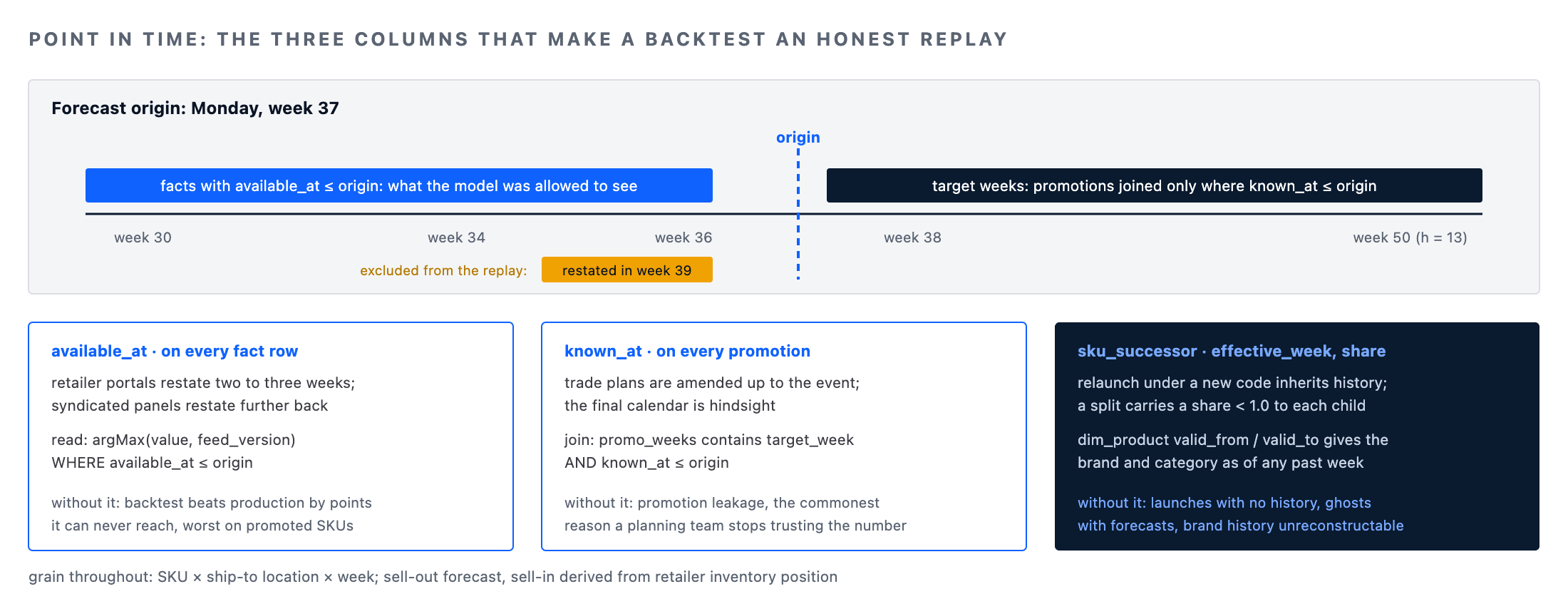
Retailer data arrives daily and is restated. A large grocer's portal will revise the previous two or three weeks as store returns, mis-scans and late polls are corrected; syndicated panel data restates further back. A demand forecasting pipeline that overwrites in place loses the ability to answer the question the accuracy review will ask: what did we know when we forecast? So the fact tables in ClickHouse are append-only with a version, and every row carries the moment it became available.
-- Demand forecasting pipeline sell-out facts: restatements append a new version; reads resolve as of a given time
CREATE TABLE cpg.pos_sales_weekly
(
    retailer_id        LowCardinality(String),
    location_id        String,                       -- retailer DC or store, per retailer feed
    sku_id             String,
    week_start         Date,
    units_sold         Decimal(18, 3),
    sales_value        Decimal(18, 2),
    on_hand_units      Nullable(Decimal(18, 3)),     -- retailer inventory where the feed provides it
    stores_selling     Nullable(UInt32),
    available_at       DateTime('UTC'),              -- when this version landed in our platform
    feed_version       UInt64                        -- monotonically increasing per feed load
)
ENGINE = ReplacingMergeTree(feed_version)
PARTITION BY toYYYYMM(week_start)
ORDER BY (retailer_id, location_id, sku_id, week_start)
SETTINGS index_granularity = 8192;

-- The point-in-time read every training set and every backtest uses
SELECT
    retailer_id, location_id, sku_id, week_start,
    argMax(units_sold,    feed_version) AS units_sold,
    argMax(on_hand_units, feed_version) AS on_hand_units,
    argMax(stores_selling, feed_version) AS stores_selling
FROM cpg.pos_sales_weekly
WHERE available_at <= {as_of:DateTime}
  AND week_start   <  {as_of_week:Date}
GROUP BY retailer_id, location_id, sku_id, week_start;
The available_at filter is the single most important line in the demand forecasting pipeline. Without it, a backtest run today sees restated history that the model in production never saw, and reports accuracy the live forecast cannot achieve. We have measured the gap at several points of WMAPE on promoted SKUs, where restatements are largest. Shipments and open orders land the same way from the ERP, and the retailer inventory feed, where one exists, is the input that later separates demand from sales during stock-outs.
Daily also means checking that the feed the demand forecasting pipeline depends on actually arrived with the expected weeks in it. A retailer portal that returns an empty file is a success to the loader and a disaster to Monday's forecast. The freshness and completeness indicators from our data quality SLOs post sit on these tables: lag of max(week_start) per retailer, and this week's row count against the trailing four-week median.
Weekly, first: rebuilding the hierarchies and calendars the demand forecasting pipeline joins to
Products in CPG are not stable. Pack sizes change, a SKU is relaunched under a new code with a new barcode, a brand is moved between categories in a portfolio review. Locations change when a retailer re-districts its DCs. A demand forecasting pipeline needs the hierarchy as it was on any past date, for training, and as it will be over the horizon, for the forecast. That is a slowly changing dimension in PostgreSQL, rebuilt weekly from the master data source, with the successor relationship that lets a new code inherit the history of the one it replaced.
-- Product hierarchy with validity, plus the successor map used to stitch history across SKU transitions
CREATE TABLE cpg.dim_product
(
    sku_id           TEXT      NOT NULL,
    valid_from       DATE      NOT NULL,
    valid_to         DATE      NOT NULL DEFAULT '9999-12-31',
    brand_id         TEXT      NOT NULL,
    category_id      TEXT      NOT NULL,
    pack_size        NUMERIC(10, 3),
    launch_week      DATE,
    CONSTRAINT dim_product_pk PRIMARY KEY (sku_id, valid_from)
);

CREATE TABLE cpg.sku_successor
(
    predecessor_sku  TEXT NOT NULL,
    successor_sku    TEXT NOT NULL,
    effective_week   DATE NOT NULL,
    history_share    NUMERIC(5, 4) NOT NULL DEFAULT 1.0,   -- < 1.0 when one SKU splits into several
    CONSTRAINT sku_successor_pk PRIMARY KEY (predecessor_sku, successor_sku),
    CONSTRAINT sku_successor_share_chk CHECK (history_share > 0 AND history_share <= 1)
);

-- Promotion calendar: one promotion per SKU and location at a time, enforced rather than assumed
CREATE EXTENSION IF NOT EXISTS btree_gist;
CREATE TABLE cpg.promo_calendar
(
    promo_id         TEXT      NOT NULL,
    sku_id           TEXT      NOT NULL,
    location_id      TEXT      NOT NULL,
    promo_weeks      DATERANGE NOT NULL,
    mechanic         TEXT      NOT NULL,     -- 'tpr', 'display', 'feature', 'multibuy'
    price_index      NUMERIC(5, 3),          -- promo price / base price, 1.000 = no discount
    known_at         DATE      NOT NULL,     -- when the trade plan recorded it; leakage guard for backtests
    CONSTRAINT promo_calendar_pk PRIMARY KEY (promo_id, sku_id, location_id),
    CONSTRAINT promo_calendar_no_overlap
        EXCLUDE USING gist (sku_id WITH =, location_id WITH =, promo_weeks WITH &&)
);
The known_at column on the promotion calendar plays the same role as available_at on the facts. A trade plan is amended right up to the event; a backtest that uses the final calendar knows about promotions that the forecast at the time did not. The demand forecasting pipeline joins promotions as of the forecast date, not as of today.
The calendar table in the demand forecasting pipeline is fiscal, not Gregorian: most CPG manufacturers plan on a 4-4-5 or 4-5-4 calendar, and the 53-week years that produces are where year-on-year features silently break. The calendar dimension carries fiscal week, the week-of-year offset to use for seasonal lags, and the distance in weeks to each holiday that moves, because Easter shifting by five weeks between years is a bigger effect on some categories than the entire promotion plan.
Weekly, second: computing features at the grain
Feature computation is where a demand forecasting pipeline spends its compute, and it belongs in the columnar store next to the facts rather than in a Python process pulling rows out. For two hundred million SKU-location-weeks, ClickHouse builds the feature table in minutes with window functions; the same job in pandas is an overnight batch that fails at 03:00 with an out-of-memory error. The features themselves are unglamorous and stable across every CPG engagement we have run.
-- Demand forecasting pipeline weekly feature build as of one origin; lag and rolling features exclude the current week
INSERT INTO cpg.features_weekly
SELECT
    s.retailer_id, s.location_id, s.sku_id, s.week_start,
    {origin_week:Date}                                              AS origin_week,
    s.units_sold,
    lagInFrame(s.units_sold, 1)  OVER w                              AS lag_1,
    lagInFrame(s.units_sold, 4)  OVER w                              AS lag_4,
    lagInFrame(s.units_sold, 13) OVER w                              AS lag_13,
    lagInFrame(s.units_sold, 52) OVER w                              AS lag_52,
    avg(s.units_sold) OVER (w ROWS BETWEEN 4  PRECEDING AND 1 PRECEDING) AS mean_4,
    avg(s.units_sold) OVER (w ROWS BETWEEN 13 PRECEDING AND 1 PRECEDING) AS mean_13,
    -- intermittency: how many of the last 13 weeks sold nothing
    sum(s.units_sold = 0) OVER (w ROWS BETWEEN 13 PRECEDING AND 1 PRECEDING) AS zero_weeks_13,
    -- distribution: stores selling as a share of the location's store count
    s.stores_selling / nullIf(l.store_count, 0)                     AS distribution_share,
    -- promotion features come from the calendar as it was known at the origin
    coalesce(p.price_index, 1.0)                                    AS price_index,
    p.mechanic IS NOT NULL                                          AS on_promo,
    -- stock-out censoring flag: sales are not demand when the shelf was empty
    s.on_hand_units = 0                                             AS oos_flag,
    dateDiff('week', d.launch_week, s.week_start)                   AS weeks_since_launch,
    c.weeks_to_easter, c.fiscal_week
FROM cpg.pos_sales_pit AS s                      -- the point-in-time view above, materialised per origin
LEFT JOIN cpg.dim_location  AS l ON l.location_id = s.location_id
LEFT JOIN cpg.promo_known   AS p ON p.sku_id = s.sku_id AND p.location_id = s.location_id
                                AND s.week_start >= p.promo_from AND s.week_start < p.promo_to
LEFT JOIN cpg.dim_product_pit AS d ON d.sku_id = s.sku_id
LEFT JOIN cpg.dim_calendar  AS c ON c.week_start = s.week_start
WINDOW w AS (PARTITION BY s.retailer_id, s.location_id, s.sku_id ORDER BY s.week_start);
Two features deserve comment. zero_weeks_13 is how the demand forecasting pipeline recognises intermittent demand, the long tail of SKU-locations that sell in some weeks and not others; a global model handles them tolerably if told, and a Croston-style baseline handles them better than seasonal naive does. oos_flag is the censoring signal: a week with zero on-hand and zero sales is not a week of zero demand, and training on it as if it were teaches the model that stock-outs are demand troughs, which then justifies the next stock-out. Where an inventory feed exists, censored weeks are either dropped from training or imputed from the location's uncensored rate.
The feature table is written per origin week rather than overwritten, which costs storage and buys reproducibility: any forecast run can be rebuilt from the features it saw. This is the same discipline as the offline store in our feature store architecture post, applied at weekly cadence.
Weekly, third: the demand forecasting pipeline run and the table it writes
The model at the centre of the demand forecasting pipeline is a single gradient-boosted model trained across all SKU-locations, with direct multi-horizon outputs for one to thirteen weeks and quantile objectives at p10, p50 and p90 rather than a point estimate. A global model beats per-series statistical models on the head of the catalogue by a wide margin, learns promotion response across similar SKUs, and copes with launches by borrowing from siblings. Seasonal naive and a Croston baseline are trained alongside, because they are what the global model must beat and what the pipeline falls back to when a segment underperforms.
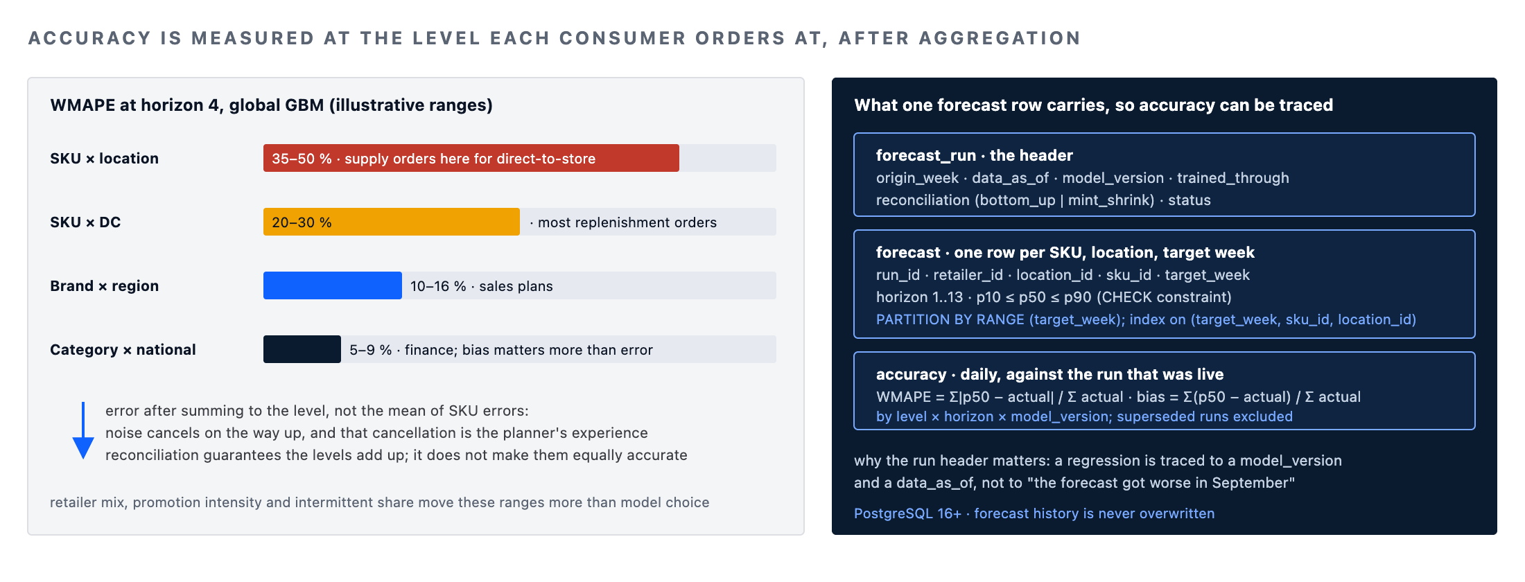
What the run writes matters more than which library trained it. Every forecast row records the run, the origin, the horizon and the model version, so that accuracy can later be measured by horizon and a regression traced to a version. The run header records what data the run saw.
-- Demand forecasting pipeline output: one header per run; one row per SKU, location, target week and horizon
CREATE TABLE cpg.forecast_run
(
    run_id            BIGINT GENERATED ALWAYS AS IDENTITY,
    origin_week       DATE        NOT NULL,           -- the Monday the forecast was cut
    data_as_of        TIMESTAMPTZ NOT NULL,           -- available_at ceiling the run used
    model_version     TEXT        NOT NULL,           -- 'gbm-2026.09.1' or 'seasonal-naive'
    trained_through   DATE        NOT NULL,
    reconciliation    TEXT        NOT NULL,           -- 'bottom_up', 'mint_shrink'
    status            TEXT        NOT NULL DEFAULT 'running',
    CONSTRAINT forecast_run_pk PRIMARY KEY (run_id),
    CONSTRAINT forecast_run_status_chk CHECK (status IN ('running','complete','failed','superseded'))
);

CREATE TABLE cpg.forecast
(
    run_id            BIGINT      NOT NULL REFERENCES cpg.forecast_run (run_id),
    retailer_id       TEXT        NOT NULL,
    location_id       TEXT        NOT NULL,
    sku_id            TEXT        NOT NULL,
    target_week       DATE        NOT NULL,
    horizon           SMALLINT    NOT NULL,           -- weeks ahead of origin, 1..13
    p10               NUMERIC(18, 3) NOT NULL,
    p50               NUMERIC(18, 3) NOT NULL,
    p90               NUMERIC(18, 3) NOT NULL,
    CONSTRAINT forecast_pk PRIMARY KEY (run_id, retailer_id, location_id, sku_id, target_week),
    CONSTRAINT forecast_quantile_chk CHECK (p10 <= p50 AND p50 <= p90)
) PARTITION BY RANGE (target_week);

CREATE INDEX forecast_target_sku_idx ON cpg.forecast (target_week, sku_id, location_id);
Reconciliation is the step that makes the demand forecasting pipeline usable by more than one function. Sales plans at brand and region, supply plans at SKU and DC, finance at category and country, and the three must agree. Forecasting each level separately and letting them disagree produces the monthly meeting where nobody's number is the number.
Bottom-up reconciliation, summing the SKU-location forecasts to every level, is simple and right when the bottom level is well-forecast; a minimum-trace approach, in the form Hyndman and Athanasopoulos describe in Forecasting: Principles and Practice, improves accuracy at the bottom by borrowing signal from the aggregates, at the cost of the planner asking why the SKU total moved. We record which was used on the run header and let the accuracy review decide.
Daily: reconciling forecast to actuals and measuring accuracy
The demand forecasting pipeline measures its own accuracy every day as actuals land, not once a month when the report is due, because a forecast that is going wrong is worth knowing about before the next run is cut. The measures are weighted absolute percentage error and bias, computed at every hierarchy level and every horizon, always against the forecast that was live for that target week at the time an order would have been placed.
-- WMAPE and bias by level and horizon, against the run that was current when the week was planned
WITH live AS (
    SELECT f.retailer_id, f.location_id, f.sku_id, f.target_week, f.horizon, f.p50,
           r.model_version
    FROM cpg.forecast f
    JOIN cpg.forecast_run r ON r.run_id = f.run_id
    WHERE r.status = 'complete'
      AND f.horizon = 4                         -- the lead time planners actually order at
      AND f.target_week >= CURRENT_DATE - INTERVAL '13 weeks'
),
joined AS (
    SELECT l.*, a.units_sold, d.brand_id, d.category_id, loc.region_id
    FROM live l
    JOIN cpg.actuals_weekly a  USING (retailer_id, location_id, sku_id, target_week)
    JOIN cpg.dim_product_current d ON d.sku_id = l.sku_id
    JOIN cpg.dim_location loc      ON loc.location_id = l.location_id
)
SELECT
    level,
    model_version,
    SUM(abs_err) / NULLIF(SUM(actual), 0)             AS wmape,
    SUM(fcst - actual) / NULLIF(SUM(actual), 0)       AS bias,
    COUNT(*)                                          AS series
FROM (
    SELECT 'sku_location' AS level, model_version,
           SUM(units_sold) AS actual, SUM(p50) AS fcst, ABS(SUM(p50) - SUM(units_sold)) AS abs_err
    FROM joined GROUP BY sku_id, location_id, model_version
    UNION ALL
    SELECT 'brand_region', model_version,
           SUM(units_sold), SUM(p50), ABS(SUM(p50) - SUM(units_sold))
    FROM joined GROUP BY brand_id, region_id, model_version
    UNION ALL
    SELECT 'category_national', model_version,
           SUM(units_sold), SUM(p50), ABS(SUM(p50) - SUM(units_sold))
    FROM joined GROUP BY category_id, model_version
) lv
GROUP BY level, model_version
ORDER BY level, model_version;
Two properties of this query are deliberate. It measures at horizon four because that is the lead time most CPG replenishment orders are placed at; a demand forecasting pipeline that reports its one-week-ahead accuracy is reporting a number nobody orders on. And it computes the error after aggregating to the level, not the average of SKU errors, because aggregation cancels noise and that cancellation is exactly what the brand planner benefits from. The two figures differ by a lot, and only one of them describes the planner's experience.
| Level, horizon 4 | Seasonal naive | Global GBM | What moves the number |
|---|---|---|---|
| SKU × location | 55–75 % | 35–50 % | Intermittency and stock-out censoring dominate; promotion features matter most here |
| SKU × DC | 35–50 % | 20–30 % | The level supply orders at; reconciliation method shows up here |
| Brand × region | 18–28 % | 10–16 % | Calendar and holiday distance; SKU transitions if the successor map is wrong |
| Category × national | 8–14 % | 5–9 % | Bias, not error: a consistent 3 % over-forecast is a warehouse of inventory by quarter end |
The ranges are illustrative of what we see across engagements, not a benchmark; the retailer mix, the promotion intensity and the share of intermittent SKUs move them by more than the model choice does. The point of the table is the shape: the demand forecasting pipeline is judged at the level each consumer uses, and improvement at the bottom compounds as it aggregates.
Monthly: backtesting the demand forecasting pipeline, champion against challenger
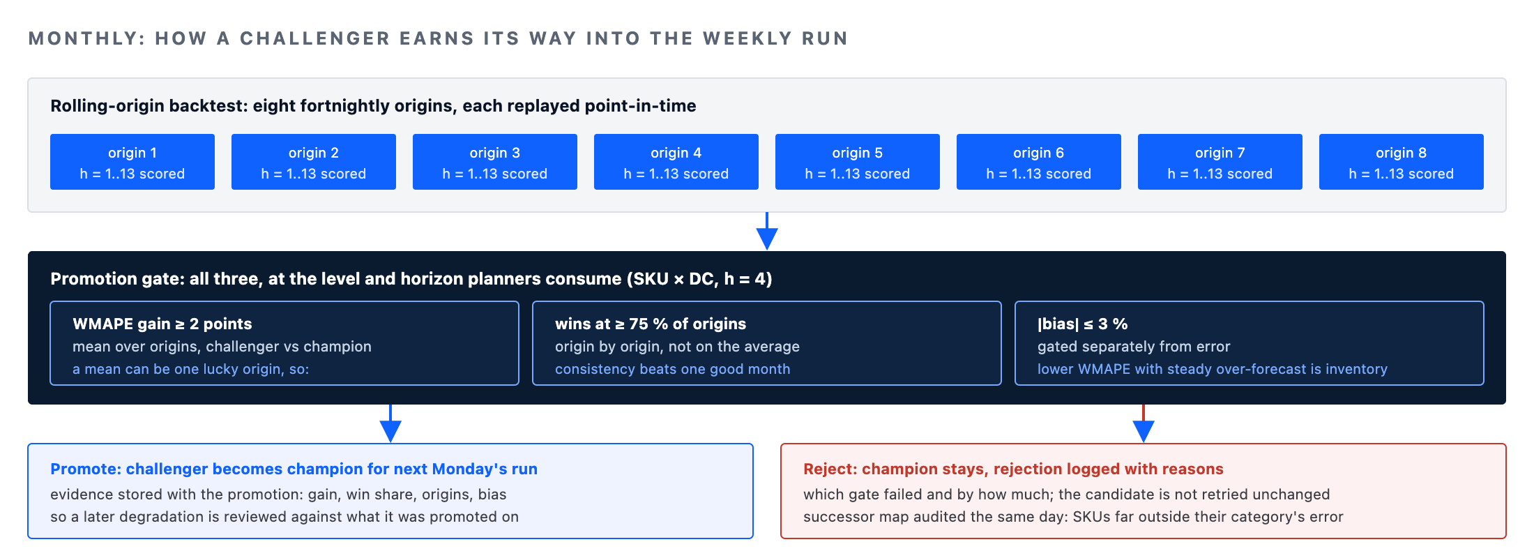
A challenger model, a new feature set or a change to the reconciliation method earns its way into production through a rolling-origin backtest: the demand forecasting pipeline is re-run from at least eight past origins, each using only data and promotion calendars available at that origin, and the challenger's accuracy is compared with the champion's at the level and horizon the planners consume. Because the facts carry available_at and the calendar carries known_at, the backtest is an honest replay rather than a reconstruction with hindsight.
# Demand forecasting pipeline rolling-origin backtest and promotion gate; runs monthly under Airflow
from datetime import date, timedelta
import pandas as pd

ORIGINS = [date(2026, 5, 4) + timedelta(weeks=i) for i in range(0, 16, 2)]   # 8 origins, fortnightly
LEVEL, HORIZON = "sku_dc", 4
GATE_WMAPE_GAIN = 0.02      # challenger must improve WMAPE by 2 points at the planning level
GATE_BIAS_ABS   = 0.03      # and keep absolute bias within 3 %

def backtest(model_version: str) -> pd.DataFrame:
    rows = []
    for origin in ORIGINS:
        feats = build_features(origin_week=origin, as_of=origin_available_at(origin))   # point-in-time
        fcst  = run_forecast(model_version, feats, horizons=range(1, 14))
        acts  = load_actuals(target_weeks=[origin + timedelta(weeks=h) for h in range(1, 14)])
        rows.append(score(fcst, acts, level=LEVEL, horizon=HORIZON).assign(origin=origin))
    return pd.concat(rows)

champ = backtest(current_champion())
chall = backtest(candidate_version())

gain = champ["wmape"].mean() - chall["wmape"].mean()
bias_ok = chall["bias"].abs().mean() <= GATE_BIAS_ABS
wins = (chall.set_index("origin")["wmape"] < champ.set_index("origin")["wmape"]).mean()

if gain >= GATE_WMAPE_GAIN and bias_ok and wins >= 0.75:
    promote(candidate_version(), evidence={"gain": gain, "wins": wins, "origins": len(ORIGINS)})
else:
    record_rejection(candidate_version(), gain=gain, wins=wins, bias_ok=bias_ok)
The gate has three parts on purpose. A mean improvement can be one lucky origin, so the challenger must also win at most origins individually. Bias is gated separately from error because a model can reduce WMAPE while introducing a consistent over-forecast, and over-forecast becomes inventory. And the evidence is written down with the promotion, so that when accuracy degrades in production the review can see what the model was promoted on. Ongoing degradation after promotion is the territory of our model drift monitoring post; the monthly backtest is the pre-promotion counterpart.
Monthly is also when the demand forecasting pipeline's successor map is audited. A SKU transition where the successor was mapped a month late shows up as a launch with no history and a discontinued item with a forecast; both are visible in the accuracy table as SKUs whose error is far outside their category.
Where a demand forecasting pipeline breaks in practice
The failures we are called in for are rarely the model. Promotion leakage, where features are built from the final trade calendar rather than the one known at the origin, produces a backtest ten points better than production and a planning team that stops trusting the number. Stock-out censoring, where a week with an empty shelf trains the model that demand was zero, produces forecasts that ratchet down after every supply problem. Hierarchy drift, where the category a SKU belonged to last year is not the one it is aggregated into today, makes brand-level history unreconstructable. And retailer restatements applied in place make last month's accuracy report unrepeatable.
Every one of those is a data problem with a table-level fix, which is why this post spends its length on schemas and cadences. A demand forecasting pipeline with available_at, known_at, a successor map and a versioned feature table is one where a better model actually produces a better number.
| Cadence | What runs | What is checked before the next step |
|---|---|---|
| Daily | Retailer, syndicated, ERP and inventory feeds appended with version and available_at; actuals reconciled to the live forecast | Feed freshness and completeness per retailer; accuracy at horizon 4 by level |
| Weekly, before the run | Hierarchy and successor rebuild; promotion calendar refreshed with known_at; fiscal calendar extended | No SKU with sales and no hierarchy row; no overlapping promotions; calendar covers the horizon |
| Weekly, the run | Feature build per origin in ClickHouse; global model and baselines; reconciliation; forecast rows written under a run header | Row count against last run; quantile ordering; totals against last run within a tolerance |
| Monthly | Rolling-origin backtest; champion and challenger; successor-map audit | Promotion gate evidence recorded; rejected candidates logged with reasons |
Working with MinervaDB on a demand forecasting pipeline
A demand forecasting pipeline is the central deliverable of our CPG data analytics practice and draws on our data engineering and MLOps consulting teams: a typical engagement starts with the grain and sell-out decision, lands the retailer feeds with point-in-time semantics, builds the hierarchy, calendar and feature layers described here, and runs the first backtest against whatever forecast the planners are using today so the improvement is measured rather than promised. The forecast tables then feed the same metrics layer the commercial teams already report from.
Under managed operations the daily feed checks, the weekly run and the monthly backtest are run by our 24×7 teams under the standard S1 to S4 commitments, with a missed weekly forecast cut treated as an S2. As always: test every schema, query and gate here against your own retailer feeds and planning calendar before applying them to production, and keep the fact and forecast tables under a tested restore posture; the history they hold is the only thing a demand forecasting pipeline cannot rebuild.
Running PostgreSQL in production? MinervaDB provides PostgreSQL consulting, 24×7 PostgreSQL support and PostgreSQL remote DBA services as part of its database consulting services.
Running this in production?
MinervaDB provides ClickHouse Consulting, Data Engineering Consulting, Data Analytics Platform Engineering and PostgreSQL Consulting with 24x7 coverage and a 15-minute S1 response. Talk to an engineer.