A feature store architecture is three contracts, not a product. The first contract is that a feature has exactly one definition, one owner and one freshness promise. The second is that any training set can be rebuilt as of any past moment without a single value leaking from the future. The third is that the number a model sees in production is the number it was trained on, computed by the same code from the same source. Every feature store we have reviewed that failed in production broke one of those three contracts, and most of the products sold under the name make it easy to break all of them quietly.
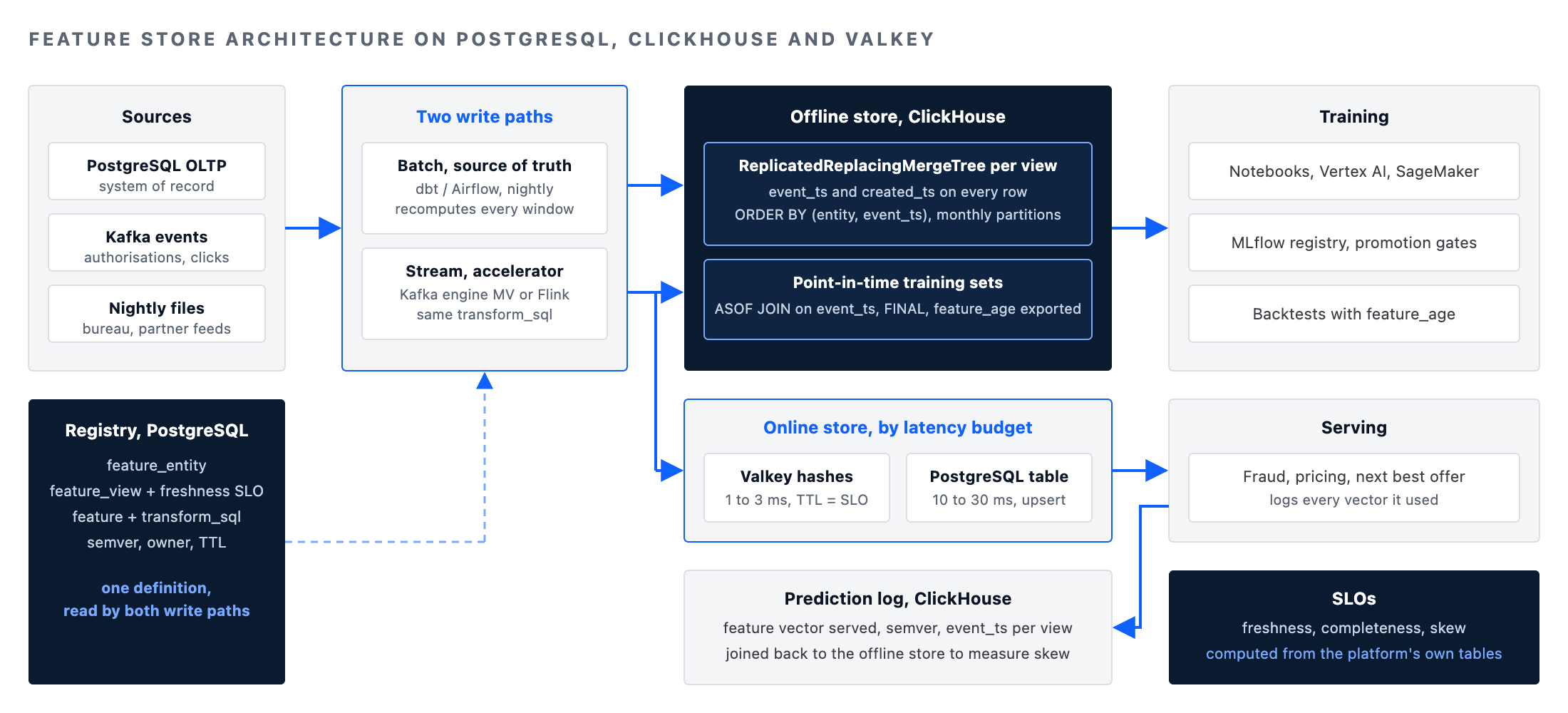
This post sets out the feature store architecture we build for teams that already run PostgreSQL for their transactional systems and want fraud, pricing, forecasting or recommendation models in production without buying a platform they cannot operate. The offline store is ClickHouse, the registry and the low-cardinality online store are PostgreSQL, and Valkey carries the hot online path where a single-digit-millisecond budget applies. It is written as seven design decisions because that is how the work actually proceeds: each decision has a failure mode we have seen, a schema or query that prevents it, and a measurement that proves it is holding. Latency and cost figures are illustrative unless a source is named.
Decision 1: the feature registry is a table, and the definition is code
The registry is where a feature store architecture either earns trust or loses it. If definitions live in notebooks and Slack threads, two teams will ship two versions of customer_30d_txn_count within a quarter, one counting authorisations and one counting settlements, and the fraud model will be trained on one and served the other. In our feature store architecture the registry lives in PostgreSQL because it is a low-volume, high-integrity workload with foreign keys, and because the people who need to query it already have access.
A feature row records the entity it keys on, the SQL or transformation reference that computes it, the event-time column that governs point-in-time joins, the freshness SLO in seconds, an owner, and a semantic version. A feature view groups features that are materialised together from one source at one grain. Nothing in the feature store architecture is materialised that is not registered, and the materialisation job reads its own instructions from this table rather than from a copy in a config repository.
-- Feature store architecture registry (PostgreSQL 16+)
CREATE TABLE feature_entity (
    entity_name        TEXT PRIMARY KEY,           -- customer, merchant, device
    join_key           TEXT NOT NULL,              -- column name in every store
    description        TEXT NOT NULL
);

CREATE TABLE feature_view (
    view_name          TEXT PRIMARY KEY,
    entity_name        TEXT NOT NULL REFERENCES feature_entity (entity_name),
    source_ref         TEXT NOT NULL,              -- dbt model or Kafka topic
    event_ts_column    TEXT NOT NULL,              -- governs point-in-time joins
    freshness_slo_sec  INTEGER NOT NULL CHECK (freshness_slo_sec > 0),
    online_enabled     BOOLEAN NOT NULL DEFAULT FALSE,
    online_ttl_sec     INTEGER,
    owner_email        TEXT NOT NULL,
    CONSTRAINT feature_view_online_ttl_chk
        CHECK (NOT online_enabled OR online_ttl_sec IS NOT NULL)
);

CREATE TABLE feature (
    view_name          TEXT NOT NULL REFERENCES feature_view (view_name),
    feature_name       TEXT NOT NULL,
    dtype              TEXT NOT NULL,              -- int64, float64, string, bool
    transform_sql      TEXT NOT NULL,              -- the single definition
    semver             TEXT NOT NULL,
    deprecated_at      TIMESTAMPTZ,
    PRIMARY KEY (view_name, feature_name)
);
The transform_sql column is the contract. The offline materialisation job templates it into a ClickHouse INSERT ... SELECT; the streaming job compiles the same expression for the online path. When a definition changes, semver moves, a new column is materialised alongside the old one, and models are re-pointed deliberately. The alternative, editing a definition in place, silently changes the training distribution of every model that depends on it.
Decision 2: the offline store keeps every value ever computed, at event time
The offline store in this feature store architecture is ClickHouse, and the reason is the shape of the workload rather than fashion. A training set for a fraud model is a point-in-time join of a few million labelled events against twenty to two hundred feature columns across a year of history. That is a wide scan with a time-ordered merge, which is exactly what MergeTree is built for, and it is a workload that will hurt a PostgreSQL primary that also has to serve the application.
Two timestamps are mandatory on every row of the feature store architecture. event_ts is when the fact became true in the world; created_ts is when the feature store learned about it. Point-in-time correctness is defined against event_ts, but the gap between the two is the feature's real-world availability lag, and a model trained on values that were not yet known at prediction time will look brilliant offline and fail on its first day. We store both and we monitor the gap.
-- Offline store: one table per feature view (ClickHouse 25.x+)
CREATE TABLE fs.customer_txn_30d
(
    customer_id            UInt64,
    event_ts               DateTime64(3, 'UTC'),
    created_ts             DateTime64(3, 'UTC') DEFAULT now64(3),
    txn_count_30d          UInt32,
    txn_amount_30d         Decimal(18, 2),
    distinct_merchants_30d UInt16,
    max_single_txn_30d     Decimal(18, 2),
    feature_semver         LowCardinality(String)
)
ENGINE = ReplicatedReplacingMergeTree(
    '/clickhouse/tables/{shard}/fs/customer_txn_30d',
    '{replica}',
    created_ts
)
PARTITION BY toYYYYMM(event_ts)
ORDER BY (customer_id, event_ts)
SETTINGS index_granularity = 8192;
ReplacingMergeTree with created_ts as the version column gives idempotent backfills: recomputing a window after a late-arriving source produces a newer row for the same key and event time, and the older one is dropped at merge. Ordering by (customer_id, event_ts) makes the ASOF join in the next decision a sequential read per customer. Partitioning by month keeps retention a metadata operation. No table in this feature store architecture is mutated in place; ALTER TABLE ... UPDATE on a feature table is the one operation we prohibit outright.
Decision 3: point-in-time joins are the only join
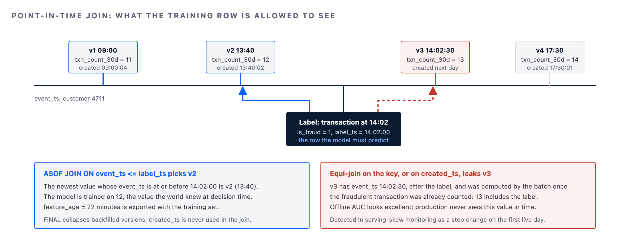
The single most common defect in a feature store architecture is label leakage through the join. A training row for a transaction at 14:02 must see the customer's feature values as they stood at 14:02, not the values recomputed at midnight after the transaction was already counted. A plain equi-join on the key does this wrong by default. An ASOF join does it right, and ClickHouse has had a native ASOF JOIN since long before it was fashionable.
-- Point-in-time training set: labels joined to features as of the label time
SELECT
    l.txn_id,
    l.customer_id,
    l.label_ts,
    l.is_fraud,
    f.txn_count_30d,
    f.txn_amount_30d,
    f.distinct_merchants_30d,
    f.max_single_txn_30d,
    f.event_ts                      AS feature_event_ts,
    l.label_ts - f.event_ts         AS feature_age
FROM fs.labels_fraud AS l
ASOF LEFT JOIN fs.customer_txn_30d FINAL AS f
    ON  f.customer_id = l.customer_id
    AND f.event_ts   <= l.label_ts
WHERE l.label_ts BETWEEN '2026-01-01' AND '2026-06-30'
SETTINGS join_algorithm = 'full_sorting_merge';
Three details carry the correctness of the feature store architecture here. FINAL collapses replaced versions so a backfill cannot produce two candidates for one moment. The inequality is <= on event_ts, never on created_ts, which is what makes the set reproducible. feature_age is exported with the training set so the modelling team can see how stale features were in training and set an alert when production staleness drifts away from it. On a 40 million label, 180 million feature-row join we have seen full_sorting_merge stay within memory where the default hash algorithm did not; check system.query_log for memory_usage and read_rows on your own data before choosing.
When the offline store is PostgreSQL alone, which is a legitimate feature store architecture for teams under a few hundred million feature rows, the same join is a LATERAL subquery with ORDER BY event_ts DESC LIMIT 1 and a composite index on (customer_id, event_ts DESC). It is correct, and it is slower by roughly an order of magnitude at scale in our measurements; EXPLAIN (ANALYZE, BUFFERS) will show whether the index-only scan holds or the planner falls back to a nested loop over heap fetches.
Decision 4: the online store is chosen by the latency budget, not by habit
The online path in a feature store architecture serves the current value of each feature for one entity, in the time the calling service can afford. That budget, not habit, decides the technology in the feature store architecture. A fraud decision inside a card authorisation typically has 20 to 50 milliseconds end to end, of which feature retrieval may take 2 to 5; a next-best-offer call on a web page has hundreds. Illustrative figures, but the shape is consistent across the estates we operate.
For the single-digit-millisecond tier we use Valkey, one hash per entity per feature view, fields named by feature, with a TTL equal to the freshness SLO so a stale value expires rather than being served. For the tier that tolerates 10 to 30 milliseconds and needs transactional semantics or joins against reference data, PostgreSQL with a narrow, heap-only-tuple-friendly table is simpler to operate and usually already present. Choosing Valkey for everything adds a cache you must keep consistent; choosing PostgreSQL for everything puts a p99-sensitive read path on the same instance as your OLTP.
-- PostgreSQL online store for the mid-latency tier: one row per entity per view,
-- overwritten in place, fill factor left low so updates stay HOT
CREATE TABLE fs_online.customer_txn_30d (
    customer_id            BIGINT PRIMARY KEY,
    event_ts               TIMESTAMPTZ NOT NULL,
    txn_count_30d          INTEGER NOT NULL,
    txn_amount_30d         NUMERIC(18, 2) NOT NULL,
    distinct_merchants_30d SMALLINT NOT NULL,
    max_single_txn_30d     NUMERIC(18, 2) NOT NULL,
    feature_semver         TEXT NOT NULL
) WITH (fillfactor = 70);

INSERT INTO fs_online.customer_txn_30d AS o
    (customer_id, event_ts, txn_count_30d, txn_amount_30d,
     distinct_merchants_30d, max_single_txn_30d, feature_semver)
VALUES ($1, $2, $3, $4, $5, $6, $7)
ON CONFLICT (customer_id) DO UPDATE
SET event_ts               = EXCLUDED.event_ts,
    txn_count_30d          = EXCLUDED.txn_count_30d,
    txn_amount_30d         = EXCLUDED.txn_amount_30d,
    distinct_merchants_30d = EXCLUDED.distinct_merchants_30d,
    max_single_txn_30d     = EXCLUDED.max_single_txn_30d,
    feature_semver         = EXCLUDED.feature_semver
WHERE EXCLUDED.event_ts > o.event_ts;   -- never move a value backwards
The WHERE EXCLUDED.event_ts > o.event_ts guard is the feature store architecture's online-store equivalent of the version column in ReplacingMergeTree: out-of-order deliveries from a stream cannot overwrite a newer value with an older one. Watch pg_stat_user_tables.n_tup_hot_upd against n_tup_upd on this table; if the HOT ratio drops, an index on a frequently updated column has crept in and autovacuum will start losing.
Decision 5: two write paths, one definition
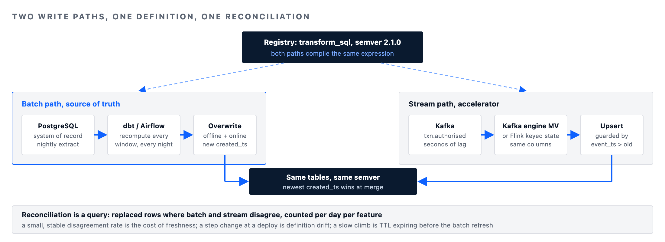
Every feature store architecture has a batch path and, for any feature that must be fresh within minutes, a streaming path. The trap is letting them drift into two definitions. Our rule is that the batch path is the source of truth and the streaming path is an accelerator: the streaming job applies the registered transformation to events from Kafka and writes to the online store and to the offline store, and the nightly batch recomputes the same windows from the system of record and overwrites both. Any disagreement between the two shows up as a replaced row in ClickHouse, and we count those.
-- Streaming ingestion into the offline store (ClickHouse Kafka engine + MV)
CREATE TABLE fs.kafka_txn_events
(
    customer_id UInt64,
    merchant_id UInt64,
    amount      Decimal(18, 2),
    event_ts    DateTime64(3, 'UTC')
)
ENGINE = Kafka
SETTINGS kafka_broker_list      = '${KAFKA_BROKERS}',
         kafka_topic_list       = 'txn.authorised',
         kafka_group_name       = 'fs-customer-txn-30d',
         kafka_format           = 'JSONEachRow',
         kafka_num_consumers    = 4,
         kafka_max_block_size   = 65536;

-- Materialised view applies the registered transform to arriving events
CREATE MATERIALIZED VIEW fs.mv_customer_txn_30d
TO fs.customer_txn_30d
AS
SELECT
    customer_id,
    max(event_ts)                                   AS event_ts,
    now64(3)                                        AS created_ts,
    count()                                         AS txn_count_30d,
    sum(amount)                                     AS txn_amount_30d,
    uniqExact(merchant_id)                          AS distinct_merchants_30d,
    max(amount)                                     AS max_single_txn_30d,
    '2.1.0'                                         AS feature_semver
FROM fs.kafka_txn_events
GROUP BY customer_id;
That view is deliberately simplified: a true rolling 30-day window needs the prior state, which in ClickHouse we keep in an AggregatingMergeTree with -State combinators and read with -Merge, and in Flink we keep as keyed state. The point of showing it is the shape: the streaming path writes rows with the same columns, the same feature_semver and a real created_ts into the same table the batch path overwrites. Reconciliation across the feature store architecture is then a query, not an investigation.
-- Batch-versus-stream disagreement rate, per day, from the replaced-row history
SELECT
    toDate(event_ts)                                            AS d,
    countIf(feature_semver_batch != '' AND txn_count_batch != txn_count_stream)
        / count()                                               AS disagreement_rate
FROM fs.customer_txn_30d_reconcile      -- built nightly from both paths
WHERE event_ts >= now() - INTERVAL 14 DAY
GROUP BY d
ORDER BY d;
Decision 6: log what the model saw, and measure skew as a number
Training and serving parity is the third contract of the feature store architecture, and it is the one nobody can verify by reading code. The only proof is data: at inference time the service writes the feature vector it actually used, with the feature_semver and the online-store event_ts for each view, to a prediction log in ClickHouse. That log is then joined, point in time, back to the offline store. Where the two disagree beyond a tolerance, the feature store architecture has a skew, and the report names the feature, the version and the hour it started.
-- Serving skew: what the model saw versus what the offline store says it should have seen
WITH served AS
(
    SELECT
        prediction_id,
        customer_id,
        served_ts,
        features['txn_count_30d']       AS txn_count_served
    FROM ml.prediction_log
    WHERE model_name = 'fraud_auth'
      AND served_ts >= now() - INTERVAL 1 DAY
)
SELECT
    toStartOfHour(s.served_ts)                                       AS h,
    count()                                                          AS predictions,
    avg(abs(s.txn_count_served - f.txn_count_30d))                   AS mean_abs_skew,
    quantile(0.99)(abs(s.txn_count_served - f.txn_count_30d))        AS p99_abs_skew,
    countIf(s.txn_count_served != f.txn_count_30d) / count()         AS mismatch_rate
FROM served AS s
ASOF LEFT JOIN fs.customer_txn_30d FINAL AS f
    ON f.customer_id = s.customer_id AND f.event_ts <= s.served_ts
GROUP BY h
ORDER BY h;
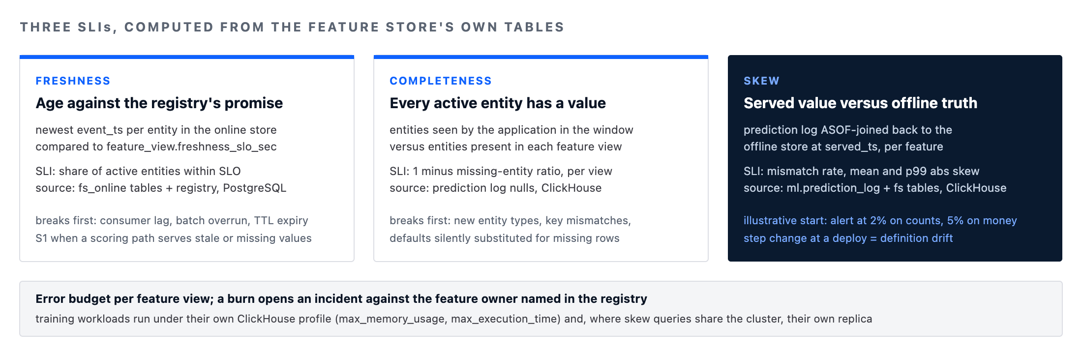
A mismatch rate that is small and stable is the normal cost of streaming freshness in any feature store architecture. A mismatch rate that steps up at a deploy is a definition drift between the two write paths. A mismatch rate that climbs slowly is usually the online TTL expiring faster than the batch path refreshes, and the fix is in the registry, not the model. Illustrative thresholds we start from: alert at 2 percent mismatch on count features, 5 percent on monetary features, then tighten against what the business tolerates.
Decision 7: operate it with SLOs, or it will be operated by incidents
A feature store architecture is a production data system, and we run it the way we run every other one: with SLOs, an error budget and a runbook per failure mode. Three SLIs cover most of what goes wrong in a feature store architecture. Freshness is the age of the newest row per entity in the online store against the registered freshness_slo_sec. Completeness is the share of active entities that have a value at all. Skew is the mismatch rate from the previous decision. Each is computed from the platform's own tables, so the monitoring cannot drift from the thing it monitors.
-- Freshness SLI per feature view, computed against the registry's own promise
SELECT
    v.view_name,
    v.freshness_slo_sec,
    EXTRACT(EPOCH FROM (now() - MAX(o.event_ts)))::INTEGER      AS newest_age_sec,
    COUNT(*) FILTER (
        WHERE now() - o.event_ts > make_interval(secs => v.freshness_slo_sec)
    )::NUMERIC / NULLIF(COUNT(*), 0)                             AS stale_entity_ratio
FROM feature_view AS v
JOIN fs_online.customer_txn_30d AS o ON TRUE     -- one query per view in practice
WHERE v.view_name = 'customer_txn_30d'
GROUP BY v.view_name, v.freshness_slo_sec;
Cost is the fourth feature store architecture number worth watching. ClickHouse compresses feature history well, typically 8 to 15 times on numeric windows in our estates, so the offline store is rarely the expensive part. Retraining queries are: an unbounded point-in-time join across a year can read terabytes, and system.query_log grouped by user and week shows which team is doing it. We give training workloads their own ClickHouse profile with max_memory_usage and max_execution_time limits, and their own replica when the serving skew queries share the cluster.
When PostgreSQL alone is the right feature store architecture
Not every team needs the three-engine feature store architecture. If total feature history is under a few hundred million rows, if training is weekly rather than continuous, and if the latency budget on the online path is above 10 milliseconds, one PostgreSQL cluster with a partitioned history table, a LATERAL point-in-time join and the online table from decision 4 is complete and operable by a team that already runs PostgreSQL. We would rather see that built well than a ClickHouse and Valkey estate built badly.
| Concern | PostgreSQL only | PostgreSQL + ClickHouse + Valkey |
|---|---|---|
| Feature history | Under ~300 M rows, partitioned by month, retained 12–18 months | Billions of rows, multi-year, 8–15× compression, S3 tiering |
| Point-in-time join | LATERAL ... ORDER BY event_ts DESC LIMIT 1; correct, index-bound | Native ASOF JOIN with sorting-merge; wide scans in minutes |
| Online p99 | 10–30 ms on a dedicated replica (illustrative) | 1–3 ms from Valkey hashes with TTL = freshness SLO (illustrative) |
| Streaming features | Micro-batch every 1–5 minutes via logical replication or Debezium | Kafka engine or Flink into the same tables, seconds of lag |
| Operational surface | One engine the team already runs; autovacuum and bloat are the risks | Three engines, Keeper quorum, cache consistency; needs a Data SRE owner |
| Right when | Weekly retraining, a handful of models, mid-latency serving | Continuous training, real-time decisions, many teams sharing features |
Where this feature store architecture needs adjusting
Three situations change the feature store architecture. Regulated estates that must prove which feature values fed a decision need the prediction log from decision 6 retained for the statutory period with the feature_semver and the registry snapshot, which turns the log into a compliance record with its own access policy.
Multi-region serving needs the online store replicated per region with the freshness SLI computed per region, because a Valkey replica lagging in one region is invisible from the other. Estates already committed to Databricks or Snowflake can keep the offline store there and still apply decisions 1, 3, 4 and 6; the registry, the point-in-time discipline and the skew measurement are portable, and they are the parts that matter.
What does not change in any feature store architecture is the order. Registry first, offline store with both timestamps second, point-in-time join before any model is trained, online store sized to a measured budget, and skew measured from the first day of serving. Teams that start a feature store architecture with the online store because it is the visible part end up rebuilding everything behind it.
Feature store architecture: questions we are asked most
Do we need Feast or a commercial feature store? Feast is a reasonable registry and SDK layer for a feature store architecture on top of exactly the stores described here, and we use it where a team wants its Python client and its feature_view abstraction. It does not remove any of the seven decisions; it gives them a vocabulary. Commercial platforms bundle the same decisions with hosting, and the trade is operational simplicity against portability and cost per feature served.
Can the offline store be the lakehouse? Yes, if the point-in-time join is fast enough for the retraining cadence. Iceberg or Delta tables queried through Spark or Trino handle the correctness; the ASOF pattern is expressed as a window function. Where teams retrain continuously, ClickHouse over the same object storage is usually the faster path for the join, and it can read Iceberg directly since 24.x.
How do we handle features from a system that only delivers nightly files? Load them with the file's business date as event_ts and the load time as created_ts. The point-in-time join will then correctly refuse to show a model the value before the file arrived, and feature_age in the training set will show the modelling team how stale that feature really is in production.
What breaks first in production? In a feature store architecture, freshness, almost always: a stream consumer lags, the batch job overruns, the online TTL expires and the model starts scoring on nulls or defaults. That is why the freshness SLI is computed from the registry's own promise and why an S1 in our support model is a scoring path serving stale or missing features, not a model with a slightly worse AUC.
Working with MinervaDB on feature store architecture
We design, build and operate feature store architecture as part of our MLOps consulting practice, usually starting with a two-week assessment of the existing feature pipeline against the three contracts, followed by a build on the customer's own PostgreSQL, ClickHouse and Valkey estate. The registry and point-in-time discipline described here also underpin our decision intelligence work, where the same features feed both models and the metrics that judge them.
Engine depth comes from the same teams that run PostgreSQL, ClickHouse and Valkey and Redis in production for our 24×7 support customers, with the freshness, completeness and skew SLIs carried into managed operations under our standard S1 to S4 response commitments. As always: test every schema and setting here against your own workload before applying it to production, and keep a tested restore and failover posture for every store in the path.
Running this in production?
MinervaDB provides ClickHouse Consulting, PostgreSQL Consulting, PostgreSQL Support and PostgreSQL Remote DBA with 24x7 coverage and a 15-minute S1 response. Talk to an engineer.