Executive brief
Databricks spend rarely runs away because the rate per DBU is wrong. It runs away because scheduled work sits on interactive compute, because clusters and warehouses stay up after the work has finished, and because a meaningful share of the invoice has no accountable owner. A Databricks FinOps workshop replaces opinion about those three problems with evidence drawn from the account’s own Databricks system tables, then converts the evidence into twelve metrics, a short list of no-regret actions and the guardrails that stop the waste returning.
What follows is the method MinervaDB uses in its Databricks FinOps workshop, written for the people who sponsor one: the platform owner, the head of data engineering and the finance partner who signs off the Databricks commitment. It covers where DBU waste hides in Databricks billing data, the developer habits that create it, how to tell whether the account is overspending, and the twelve metrics we ask a steering committee to adopt. All SQL runs against Unity Catalog system tables, and all cost is derived from system.billing.list_prices, so nothing depends on a rate card that changes by cloud, region, tier and contract.
Why DBU Waste Hides in Databricks Billing
Databricks billing is precise and still hard to read. Each record in system.billing.usage says how many DBUs a SKU consumed in a time window, attributed to a workspace and, where it applies, to a cluster, job run, warehouse, pipeline or serving endpoint. On classic compute, a second bill from the cloud provider covers the virtual machines, disks and networking underneath. Serverless SKUs fold that infrastructure into a higher DBU rate. None of this is hidden; it is simply spread across two invoices, dozens of SKUs and hundreds of owners, which is why nobody sees the pattern without deliberately assembling it.
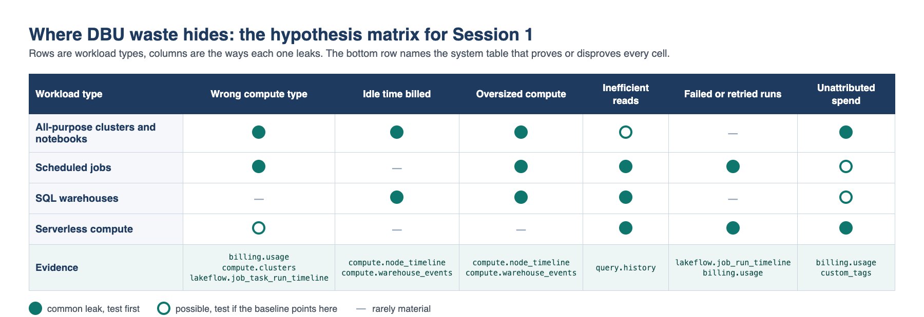
Databricks overspending concentrates in a small number of places, and each workload type leaks in its own way. The matrix below is the hypothesis we test in the first session; the system tables either confirm each cell or rule it out.
Before the Workshop: Access and Evidence
A Databricks FinOps workshop runs on the client’s data, not on samples, so the only pre-work is access. The billing schema is available by default; the compute, lakeflow and query schemas must be enabled by an account admin before they collect data, which is worth doing several weeks ahead of the first session. Read access to the Databricks system tables is granted to a dedicated group and revoked at the end.
-- Run as a metastore admin. `finops_workshop` is a dedicated account group.
GRANT USE CATALOG ON CATALOG system TO `finops_workshop`;

GRANT USE SCHEMA ON SCHEMA system.billing  TO `finops_workshop`;
GRANT SELECT     ON SCHEMA system.billing  TO `finops_workshop`;

GRANT USE SCHEMA ON SCHEMA system.compute  TO `finops_workshop`;
GRANT SELECT     ON SCHEMA system.compute  TO `finops_workshop`;

GRANT USE SCHEMA ON SCHEMA system.lakeflow TO `finops_workshop`;
GRANT SELECT     ON SCHEMA system.lakeflow TO `finops_workshop`;

GRANT USE SCHEMA ON SCHEMA system.query    TO `finops_workshop`;
GRANT SELECT     ON SCHEMA system.query    TO `finops_workshop`;

-- At close of engagement, revoke in the same order with REVOKE ... FROM `finops_workshop`.
system.query.history returns statement text only to account admins and members of the PII-access group; the workshop does not need it, because every metric below works on metadata columns. Retention matters for planning: billing and most compute, job and query tables keep 365 days, while the minute-level system.compute.node_timeline keeps 90.
Session 1: A Priced, Attributed Baseline of Databricks Billing
The first session of the Databricks FinOps workshop produces one table the whole steering committee agrees on: list cost for the last 30 days, by product and SKU, with the share each contributes. Corrections in system.billing.usage arrive as RETRACTION and RESTATEMENT records, so the query aggregates rather than reading rows individually.
WITH priced AS (
    SELECT
        u.*,
        u.usage_quantity
          * CAST(lp.pricing.effective_list.default AS DECIMAL(38, 10)) AS list_cost_usd
    FROM system.billing.usage AS u
    JOIN system.billing.list_prices AS lp
        ON  u.sku_name   = lp.sku_name
        AND u.cloud      = lp.cloud
        AND u.usage_unit = lp.usage_unit
        AND u.usage_start_time >= lp.price_start_time
        AND (lp.price_end_time IS NULL OR u.usage_start_time < lp.price_end_time)
    WHERE u.usage_date >= DATE_SUB(CURRENT_DATE(), 30)
)
SELECT
    billing_origin_product,
    sku_name,
    ROUND(SUM(usage_quantity), 1)                                            AS dbus,
    ROUND(SUM(list_cost_usd), 2)                                             AS list_cost_usd,
    ROUND(100 * SUM(list_cost_usd) / SUM(SUM(list_cost_usd)) OVER (), 1)     AS pct_of_total
FROM priced
GROUP BY billing_origin_product, sku_name
HAVING SUM(usage_quantity) <> 0
ORDER BY list_cost_usd DESC;
The second artefact from Session 1 is the rate comparison that frames most Databricks cost optimization decisions. Published list prices put all-purpose compute at a multiple of jobs compute per DBU on the same hardware; the exact ratio for the account comes from its own price table, and committed-use discounts move both SKUs together, so the ratio survives any contract.
SELECT
    sku_name,
    CAST(pricing.effective_list.default AS DECIMAL(10, 4)) AS usd_per_dbu
FROM system.billing.list_prices
WHERE price_end_time IS NULL
  AND usage_unit = 'DBU'
  AND (sku_name LIKE '%JOBS%' OR sku_name LIKE '%ALL_PURPOSE%')
ORDER BY sku_name;
Session 2: A Databricks Cost Optimization Clinic for Developers
The second session is a working clinic with engineering leads. The point is not to assign blame; most of these habits are rational choices made under delivery pressure, which is exactly why they persist. Each row below names the Databricks system tables evidence that confirms it, and a fix that does not slow the team down.
| Anti-pattern | Why it costs money | Evidence | Durable fix |
|---|---|---|---|
| Scheduling a notebook against the interactive cluster it was written on | Bills at the all-purpose rate for the life of the job, and keeps the cluster warm between runs | job_task_run_timeline.compute_ids joined to clusters.cluster_source | Job compute or serverless jobs; policy that blocks scheduling on interactive clusters |
| Auto-termination set long, or set to 0 | Idle minutes bill on both the Databricks and the cloud invoice | clusters.autotermination_minutes | Compute policy with a fixed range |
| Clusters sized for the month-end peak | Every other day runs at peak size | node_timeline p95 CPU and memory | Narrower autoscaling range; separate peak job |
| Photon switched on by default | Higher DBU rate without a matching runtime reduction on UDF-bound code | Cost per run before and after, per job | Enable per workload on measured benefit |
| Warehouses with long auto-stop and dashboards refreshing every few minutes | Warehouse never stops | warehouse_events against query.history | Shorter auto-stop; refresh schedules aligned to data arrival |
| Small files and unclustered Delta tables | Each query reads more data, so runs longer | read_files, pruned_files, read_bytes | Table maintenance and clustering on the hottest tables |
| Retrying a failing job without fixing it | Every attempt consumes DBUs and produces nothing | job_run_timeline.result_state with priced usage | Retry limits plus an owner alert on repeated failure |
| Reading only the DBU line | Spot mix, disks and egress on the cloud bill are invisible | Cloud billing export, joined on propagated cluster tags | Shared tag standard across both invoices |
The single most valuable query in the clinic, and the quickest Databricks cost optimization win, finds jobs running on all-purpose clusters, because the fix is mechanical and the saving is immediate:
WITH all_purpose AS (
    SELECT workspace_id, cluster_id, cluster_name
    FROM system.compute.clusters
    WHERE cluster_source IN ('UI', 'API')
    QUALIFY ROW_NUMBER() OVER (PARTITION BY workspace_id, cluster_id
                               ORDER BY change_time DESC) = 1
),
task_compute AS (
    SELECT workspace_id, job_id, job_run_id, EXPLODE(compute_ids) AS compute_id
    FROM system.lakeflow.job_task_run_timeline
    WHERE period_start_time >= CURRENT_TIMESTAMP() - INTERVAL 30 DAYS
)
SELECT
    t.workspace_id,
    t.job_id,
    a.cluster_name,
    COUNT(DISTINCT t.job_run_id) AS runs_on_all_purpose
FROM task_compute AS t
JOIN all_purpose AS a
    ON  a.workspace_id = t.workspace_id
    AND a.cluster_id   = t.compute_id
GROUP BY ALL
ORDER BY runs_on_all_purpose DESC;
The Databricks Overspending Test: Five Questions for the Steering Committee
Databricks overspending is a judgement about value, not a number, so the workshop frames it as five questions. Two or more answers of “no” or “we don’t know” is, in our assessment, sufficient evidence that the account is spending more than it needs to.
- Can every dollar of last month’s list cost be assigned to a named owner? If attribution is below roughly nine dollars in ten, governance is operating on partial information.
- Is cost per unit of business output flat or falling while volume grows? Rising unit cost during growth means configuration, not demand, is driving spend.
- Is scheduled work on job or serverless compute rather than all-purpose clusters? Any recurring job on interactive compute fails the test.
- Do clusters and warehouses spend most of their billed time doing work? Low p95 utilization and low query-hours per uptime-hour say they do not.
- Will the Databricks commitment land within its tolerance band? Material under- or over-consumption is a forecasting failure that finance will price into the next negotiation.
Session 3: The 12 Metrics That Expose Costly DBU Waste
The twelve metrics are grouped into four lenses so that each has an obvious owner: finance owns allocation, the platform team owns compute efficiency, engineering leads own workload efficiency, and the platform owner owns governance. Every metric names its source in the Databricks system tables and can be refreshed on a schedule without the workshop team present. Together they become the backbone of Databricks cost monitoring after the workshop ends.
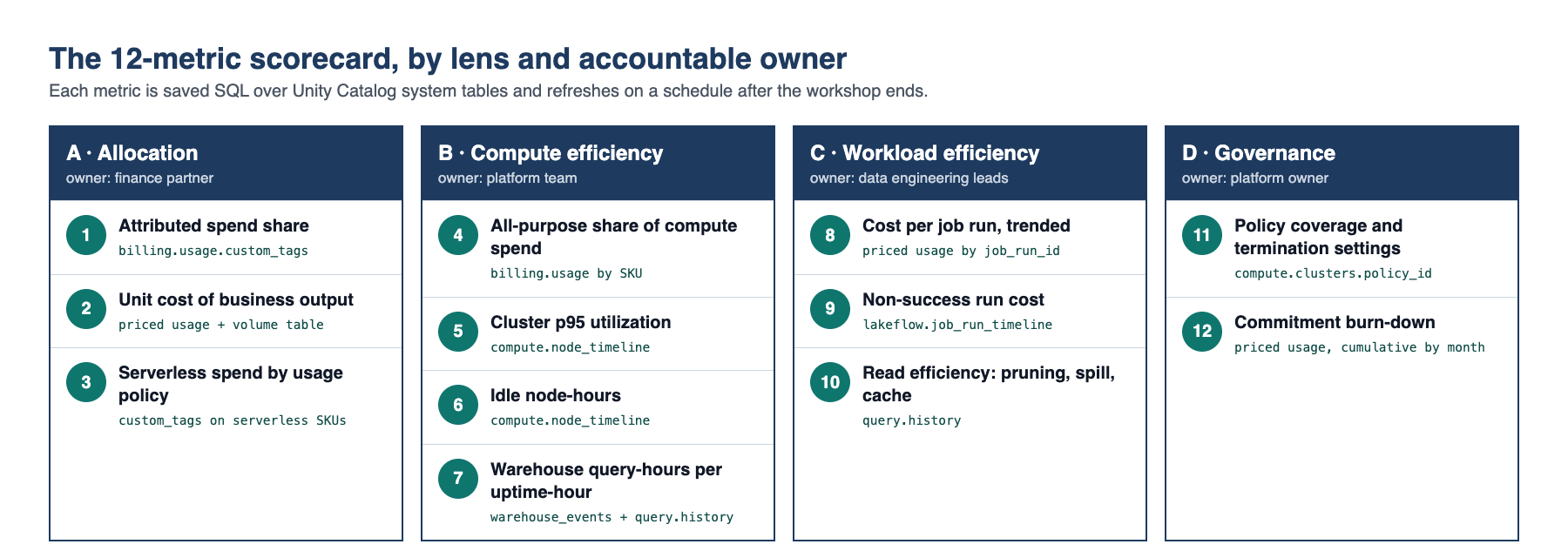
| # | Metric | Question it answers | Source | Review trigger |
|---|---|---|---|---|
| 1 | Attributed spend share | Who owns the money? | billing.usage.custom_tags | Falls below the agreed floor |
| 2 | Unit cost of output | Is spend growing faster than value? | Priced usage plus a business volume table | Rises two months running |
| 3 | Serverless spend by usage policy | Is serverless attributable and justified? | custom_tags on serverless SKUs | Untagged serverless spend appears |
| 4 | All-purpose share of compute spend | Is scheduled work on the right compute? | billing.usage by SKU | High and flat month over month |
| 5 | Cluster p95 utilization | Are clusters the right size? | compute.node_timeline | Low p95 over 14 days |
| 6 | Idle node-hours | How much compute bills while doing nothing? | compute.node_timeline | Any sustained idle pattern |
| 7 | Warehouse query-hours per uptime-hour | Are SQL warehouses earning their uptime? | compute.warehouse_events, query.history | Ratio near zero |
| 8 | Cost per job run, trended | Is each pipeline getting more expensive? | Priced usage by job_run_id | Weekly median rises |
| 9 | Non-success run cost | What do failures cost? | lakeflow.job_run_timeline | Recurring failures with retries |
| 10 | Read efficiency | Do queries read only what they need? | query.history | Low pruning ratio, high spill |
| 11 | Policy coverage | Is classic compute governed? | compute.clusters.policy_id | Clusters without a policy |
| 12 | Commitment burn-down | Will the contract land as forecast? | Priced usage, cumulative by month | Outside the tolerance band |
Lens A: Allocation and accountability (metrics 1 to 3)
In Databricks billing, allocation comes first because every other conversation depends on it. Metric 1 is the share of list cost carrying the organisation’s ownership tag. Metric 3 applies the same test to serverless SKUs, whose tags come from serverless usage policies rather than cluster configuration but land in the same custom_tags column.
WITH priced AS (
    SELECT
        u.*,
        u.usage_quantity
          * CAST(lp.pricing.effective_list.default AS DECIMAL(38, 10)) AS list_cost_usd
    FROM system.billing.usage AS u
    JOIN system.billing.list_prices AS lp
        ON  u.sku_name   = lp.sku_name
        AND u.cloud      = lp.cloud
        AND u.usage_unit = lp.usage_unit
        AND u.usage_start_time >= lp.price_start_time
        AND (lp.price_end_time IS NULL OR u.usage_start_time < lp.price_end_time)
    WHERE u.usage_date >= DATE_SUB(CURRENT_DATE(), 30)
)
SELECT
    CASE WHEN sku_name LIKE '%SERVERLESS%' THEN 'serverless' ELSE 'classic' END AS compute_class,
    ROUND(SUM(list_cost_usd), 2)                                              AS list_cost_usd,
    ROUND(100 * SUM(CASE WHEN custom_tags['cost_center'] IS NOT NULL
                         THEN list_cost_usd END) / SUM(list_cost_usd), 1)     AS pct_attributed
FROM priced
GROUP BY 1
ORDER BY list_cost_usd DESC;
Metric 2, unit cost, needs a denominator the CFO recognises: rows ingested, pipelines delivered on SLA, models scored, active analysts. Most organisations already hold that number somewhere; the workshop lands it in a small table and joins it by day.
WITH priced AS (
    SELECT
        u.*,
        u.usage_quantity
          * CAST(lp.pricing.effective_list.default AS DECIMAL(38, 10)) AS list_cost_usd
    FROM system.billing.usage AS u
    JOIN system.billing.list_prices AS lp
        ON  u.sku_name   = lp.sku_name
        AND u.cloud      = lp.cloud
        AND u.usage_unit = lp.usage_unit
        AND u.usage_start_time >= lp.price_start_time
        AND (lp.price_end_time IS NULL OR u.usage_start_time < lp.price_end_time)
    WHERE u.usage_date >= DATE_SUB(CURRENT_DATE(), 90)
),
daily_cost AS (
    SELECT usage_date, SUM(list_cost_usd) AS list_cost_usd
    FROM priced
    GROUP BY usage_date
)
SELECT
    DATE_TRUNC('MONTH', c.usage_date)                                  AS month,
    ROUND(SUM(c.list_cost_usd), 2)                                     AS list_cost_usd,
    SUM(v.rows_ingested)                                               AS rows_ingested,
    ROUND(SUM(c.list_cost_usd) / NULLIF(SUM(v.rows_ingested) / 1e9, 0), 2) AS usd_per_billion_rows
FROM daily_cost AS c
JOIN finops.business_volume AS v      -- your own daily volume table
    ON v.volume_date = c.usage_date
GROUP BY 1
ORDER BY 1;
Lens B: Compute efficiency (metrics 4 to 7)
Compute efficiency is typically the largest Databricks cost optimization lever on classic workloads. Metric 4 falls straight out of the Session 1 baseline. Metrics 5 and 6 come from system.compute.node_timeline, which records CPU, memory and network per node per minute for classic all-purpose and jobs compute. One query yields both: p95 utilization for sizing decisions and the count of node-minutes spent close to idle.
SELECT
    cluster_id,
    driver,
    COUNT(*)                                                                   AS node_minutes,
    ROUND(PERCENTILE(cpu_user_percent + cpu_system_percent, 0.95), 1)          AS p95_cpu_pct,
    ROUND(PERCENTILE(mem_used_percent, 0.95), 1)                               AS p95_mem_pct,
    ROUND(SUM(CASE WHEN cpu_user_percent + cpu_system_percent < 5
                   THEN 1 ELSE 0 END) / 60.0, 1)                               AS idle_node_hours
FROM system.compute.node_timeline
WHERE start_time >= CURRENT_TIMESTAMP() - INTERVAL 14 DAYS
GROUP BY cluster_id, driver
HAVING COUNT(*) > 600
ORDER BY idle_node_hours DESC;
The 5% CPU threshold for “idle” is a starting assumption; agree it with the platform team and keep it fixed so the trend is comparable. Metric 7 covers SQL warehouses, which node_timeline does not: uptime from system.compute.warehouse_events against query time from system.query.history. Concurrency means a busy warehouse can exceed one query-hour per uptime-hour; a value near zero means it is mostly waiting.
WITH events AS (
    SELECT
        warehouse_id,
        event_type,
        event_time,
        LEAD(event_time) OVER (PARTITION BY warehouse_id ORDER BY event_time) AS next_event_time
    FROM system.compute.warehouse_events
    WHERE event_time >= CURRENT_TIMESTAMP() - INTERVAL 7 DAYS
),
uptime AS (
    SELECT
        warehouse_id,
        SUM(TIMESTAMPDIFF(SECOND, event_time,
                          COALESCE(next_event_time, CURRENT_TIMESTAMP()))) / 3600.0 AS up_hours
    FROM events
    WHERE event_type IN ('RUNNING', 'SCALED_UP', 'SCALED_DOWN')
    GROUP BY warehouse_id
),
busy AS (
    SELECT
        compute.warehouse_id               AS warehouse_id,
        SUM(total_duration_ms) / 3600000.0 AS query_hours
    FROM system.query.history
    WHERE compute.type = 'WAREHOUSE'
      AND start_time >= CURRENT_TIMESTAMP() - INTERVAL 7 DAYS
    GROUP BY compute.warehouse_id
)
SELECT
    u.warehouse_id,
    ROUND(u.up_hours, 1)                                          AS up_hours,
    ROUND(COALESCE(b.query_hours, 0), 1)                          AS query_hours,
    ROUND(COALESCE(b.query_hours, 0) / NULLIF(u.up_hours, 0), 2)  AS query_hours_per_up_hour
FROM uptime AS u
LEFT JOIN busy AS b
    ON b.warehouse_id = u.warehouse_id
ORDER BY query_hours_per_up_hour ASC;
Lens C: Workload efficiency (metrics 8 to 10)
Workload metrics belong to the engineering leads who own the pipelines, and they make Databricks overspending visible one pipeline at a time. Metrics 8 and 9 share one query: priced usage per job run, joined to the run’s outcome, trended weekly. A rising median cost per successful run is an early warning of data growth, skew or a regression; spend on non-successful runs is pure waste.
WITH priced AS (
    SELECT
        u.*,
        u.usage_quantity
          * CAST(lp.pricing.effective_list.default AS DECIMAL(38, 10)) AS list_cost_usd
    FROM system.billing.usage AS u
    JOIN system.billing.list_prices AS lp
        ON  u.sku_name   = lp.sku_name
        AND u.cloud      = lp.cloud
        AND u.usage_unit = lp.usage_unit
        AND u.usage_start_time >= lp.price_start_time
        AND (lp.price_end_time IS NULL OR u.usage_start_time < lp.price_end_time)
    WHERE u.usage_date >= DATE_SUB(CURRENT_DATE(), 60)
),
run_cost AS (
    SELECT
        workspace_id,
        usage_metadata.job_id      AS job_id,
        usage_metadata.job_run_id  AS run_id,
        MIN(usage_start_time)      AS first_usage_time,
        SUM(list_cost_usd)         AS cost_usd
    FROM priced
    WHERE billing_origin_product = 'JOBS'
    GROUP BY ALL
),
run_outcome AS (
    SELECT workspace_id, job_id, run_id, MAX(result_state) AS result_state
    FROM system.lakeflow.job_run_timeline
    WHERE period_start_time >= CURRENT_TIMESTAMP() - INTERVAL 60 DAYS
    GROUP BY ALL
)
SELECT
    c.workspace_id,
    c.job_id,
    DATE_TRUNC('WEEK', c.first_usage_time)                                    AS week,
    COUNT(*)                                                                  AS runs,
    ROUND(PERCENTILE(CASE WHEN o.result_state = 'SUCCEEDED' THEN c.cost_usd END, 0.5), 2)
                                                                              AS median_success_run_usd,
    ROUND(SUM(CASE WHEN o.result_state <> 'SUCCEEDED' THEN c.cost_usd END), 2) AS non_success_usd
FROM run_cost AS c
LEFT JOIN run_outcome AS o
    ON  o.workspace_id = c.workspace_id
    AND o.job_id       = c.job_id
    AND o.run_id       = c.run_id
GROUP BY ALL
ORDER BY c.job_id, week;
Metric 10, read efficiency, is where table design meets Databricks billing. system.query.history records bytes read, files read and pruned, local spill and result-cache hits for every statement on SQL warehouses and serverless compute.
SELECT
    compute.warehouse_id                                                AS warehouse_id,
    COUNT(*)                                                            AS statements,
    ROUND(SUM(read_bytes) / POWER(1024, 4), 2)                          AS tb_read,
    ROUND(100 * SUM(pruned_files)
              / NULLIF(SUM(pruned_files) + SUM(read_files), 0), 1)      AS pct_files_pruned,
    ROUND(SUM(spilled_local_bytes) / POWER(1024, 3), 1)                 AS gb_spilled,
    ROUND(100 * AVG(CASE WHEN from_result_cache THEN 1 ELSE 0 END), 1)  AS pct_from_cache
FROM system.query.history
WHERE start_time >= CURRENT_TIMESTAMP() - INTERVAL 7 DAYS
  AND execution_status = 'FINISHED'
GROUP BY compute.warehouse_id
ORDER BY tb_read DESC;
Lens D: Governance and commercial control (metrics 11 and 12)
Metric 11 measures how much classic compute is actually governed: the share of interactive clusters created under a compute policy, and how many still run with termination disabled or set long. Policy coverage is the leading indicator for metrics 4 to 6, because a policy is what stops a fixed finding from quietly reappearing.
WITH latest AS (
    SELECT *
    FROM system.compute.clusters
    WHERE cluster_source IN ('UI', 'API')
      AND delete_time IS NULL
    QUALIFY ROW_NUMBER() OVER (PARTITION BY workspace_id, cluster_id
                               ORDER BY change_time DESC) = 1
)
SELECT
    workspace_id,
    COUNT(*)                                                                  AS interactive_clusters,
    ROUND(100 * AVG(CASE WHEN policy_id IS NOT NULL THEN 1 ELSE 0 END), 1)    AS pct_on_policy,
    SUM(CASE WHEN autotermination_minutes = 0 THEN 1 ELSE 0 END)              AS never_terminate,
    SUM(CASE WHEN autotermination_minutes > 60 THEN 1 ELSE 0 END)             AS terminate_after_60_plus
FROM latest
GROUP BY workspace_id
ORDER BY pct_on_policy ASC;
Metric 12 is the part of Databricks cost monitoring that finance reads first. Databricks budgets send email alerts at up to four monthly thresholds, filtered by workspace and tag, but they do not stop general compute spend and can trail usage by up to a day. The burn-down is therefore computed directly, as cumulative list cost against the committed amount; substitute the contract’s effective discount if list price is not how the commitment is drawn down.
WITH priced AS (
    SELECT
        u.*,
        u.usage_quantity
          * CAST(lp.pricing.effective_list.default AS DECIMAL(38, 10)) AS list_cost_usd
    FROM system.billing.usage AS u
    JOIN system.billing.list_prices AS lp
        ON  u.sku_name   = lp.sku_name
        AND u.cloud      = lp.cloud
        AND u.usage_unit = lp.usage_unit
        AND u.usage_start_time >= lp.price_start_time
        AND (lp.price_end_time IS NULL OR u.usage_start_time < lp.price_end_time)
    WHERE u.usage_date >= DATE_SUB(CURRENT_DATE(), 365)
),
monthly AS (
    SELECT DATE_TRUNC('MONTH', usage_date) AS month, SUM(list_cost_usd) AS list_cost_usd
    FROM priced
    WHERE usage_date >= :contract_start_date
    GROUP BY 1
)
SELECT
    month,
    ROUND(list_cost_usd, 2)                                                    AS month_usd,
    ROUND(SUM(list_cost_usd) OVER (ORDER BY month), 2)                         AS cumulative_usd,
    ROUND(100 * SUM(list_cost_usd) OVER (ORDER BY month) / :annual_commit_usd, 1) AS pct_of_commit
FROM monthly
ORDER BY month;
Session 4: Guardrails, Ownership and Cadence
Databricks FinOps workshop findings decay unless the platform enforces them and someone owns them. Session 4 turns the scorecard into controls. The compute policy below is the template we start from for Databricks cost optimization on interactive development compute: termination in a narrow range, a DBU-per-hour ceiling, required ownership tags and spot workers with on-demand fallback. The values are illustrative and are set from the account’s own metric 5 and 6 results.
{
  "cluster_type":                { "type": "fixed", "value": "all-purpose" },
  "autotermination_minutes":     { "type": "range", "minValue": 10, "maxValue": 30, "defaultValue": 20 },
  "dbus_per_hour":               { "type": "range", "maxValue": 20 },
  "autoscale.min_workers":       { "type": "fixed", "value": 1, "hidden": true },
  "autoscale.max_workers":       { "type": "range", "maxValue": 6, "defaultValue": 4 },
  "custom_tags.cost_center":     { "type": "unlimited", "isOptional": false },
  "custom_tags.owner":           { "type": "unlimited", "isOptional": false },
  "aws_attributes.availability": { "type": "fixed", "value": "SPOT_WITH_FALLBACK" }
}
Roll new policies out to development workspaces first, assign them to groups rather than individuals, and keep the previous definition as the rollback. Existing clusters are checked against a changed policy at their next edit, so announce the change before it lands. Cluster and warehouse configuration changes restart compute, so schedule them in agreed windows; test on your own workload before production and keep a tested recovery path in place.
Ownership is written down rather than assumed. The accountability matrix we leave behind for Databricks cost monitoring is deliberately short:
| Activity | Platform owner | Data engineering leads | Finance partner | Workspace admins |
|---|---|---|---|---|
| Tag standard and serverless usage policies | Accountable | Consulted | Consulted | Responsible |
| Compute policies and termination ranges | Accountable | Consulted | Informed | Responsible |
| Job compute type, retries and run cost | Informed | Accountable and responsible | Informed | Consulted |
| Warehouse sizing and auto-stop | Accountable | Consulted | Informed | Responsible |
| Budgets, thresholds and commitment forecast | Consulted | Informed | Accountable and responsible | Consulted |
| Weekly scorecard review | Accountable | Responsible | Responsible | Consulted |
What the Steering Committee Receives
The Databricks FinOps workshop closes with a readout to the steering committee and leaves four artefacts with the client: the priced and attributed baseline from Session 1; a findings register built from the Session 2 clinic, with evidence, estimated list-price impact, effort and risk for each item; the twelve-metric scorecard as saved SQL ready to schedule; and the guardrail pack from Session 4, staged for rollout from development to production. Recommendations are sequenced so that no-regret changes, such as moving scheduled jobs off interactive compute, come first, and changes that need performance testing, such as Photon or warehouse resizing, follow with measurement.
Three questions tend to come up when scoping a Databricks FinOps workshop. Databricks system tables are free to retain but not free to query, because queries run on the account’s own compute, so scheduled scorecard refreshes belong on a small warehouse. Serverless is not automatically cheaper in Databricks billing terms; it removes idle time and bundles infrastructure into the rate, so it is compared on total cost per run with both invoices included. And poor tagging does not block the work: workspace, job and warehouse identifiers in usage_metadata support a first allocation while the tag standard is fixed.
Schedule a Databricks FinOps Workshop
If Databricks spend is growing faster than the value it produces, the fastest route from debate to decision is a Databricks FinOps workshop on your own system tables. MinervaDB’s Databricks consulting and 24×7 support practice runs it for platform, engineering and finance leads together, and it complements the cross-platform controls in our Snowflake and Databricks FinOps guide. Contact us to scope a session.
Databricks Documentation Used in This Workshop
- System tables overview
- Billable usage
- Pricing table
- Compute tables
- Warehouse events
- Jobs tables
- Query history
- Compute policy reference
- Budgets
- Serverless usage policies
- FinOps Foundation framework
Running this in production?
MinervaDB provides Databricks Consulting and Data Analytics Platform Engineering with 24x7 coverage and a 15-minute S1 response. Talk to an engineer.