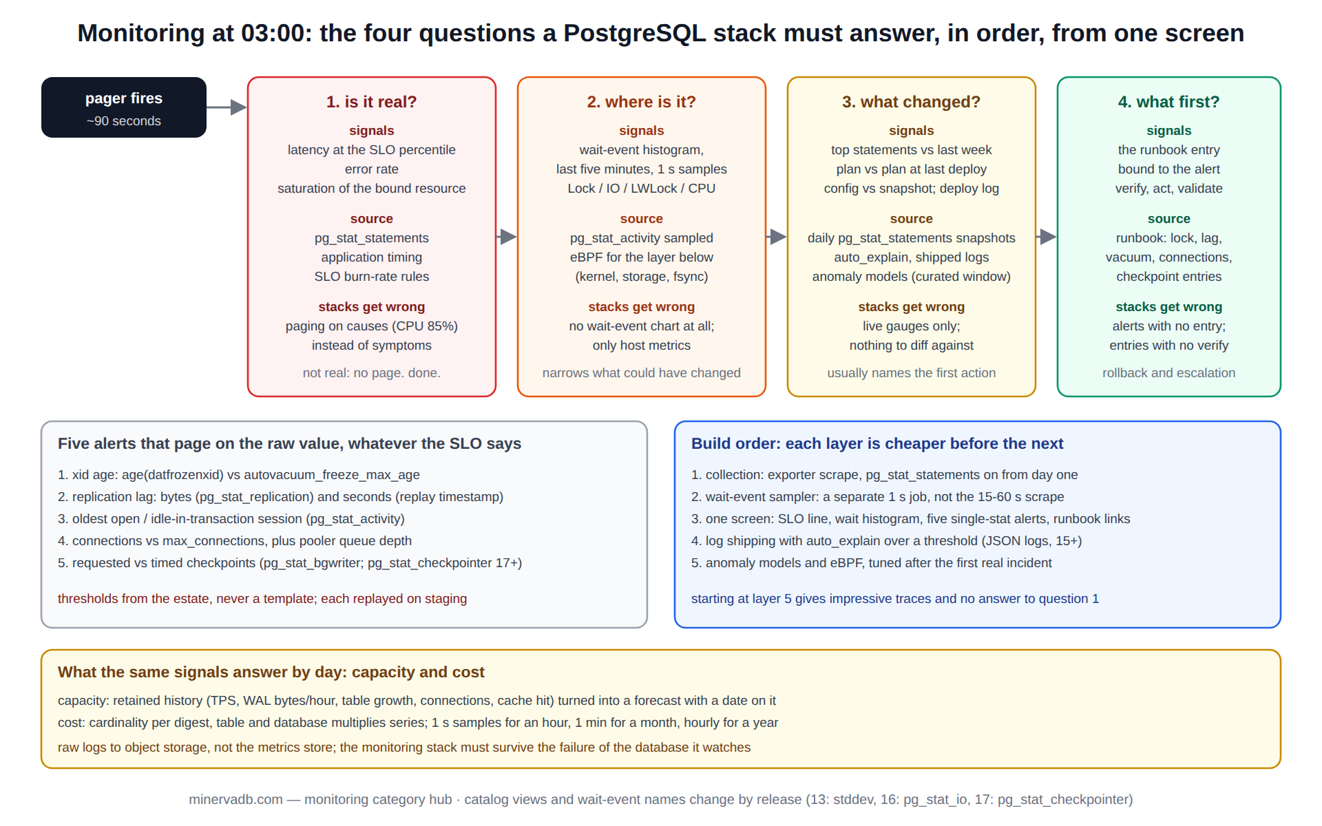
A monitoring stack is judged at three in the morning, not in the demo. The pager has fired, the engineer on call has one eye open, and the stack has about ninety seconds to answer four questions in order: is it real, where is it, what changed, and what do we do first. A stack that answers all four from a single screen ends the incident before the customer notices; a stack that answers only the first one produces a war room.
Everything else about database monitoring, the exporters, the dashboards, the log pipeline, the anomaly models, is a means to those four answers.
This page organises a PostgreSQL monitoring practice around the four questions. Each section states the question, names the signals that answer it, the catalog views and tools that produce those signals, and the archive post that shows the setup in detail. The order is deliberate: it is the order the on-call engineer needs them in, and it is the order MinervaDB uses when auditing a customer’s monitoring, because a stack with beautiful capacity dashboards and no lock-wait alert has answered question four and skipped question one.
The archive it introduces covers wait-event analysis, Prometheus and postgres_exporter, Grafana dashboards, pgBadger, Datadog, pganalyze, eBPF tracing, SLO-based alerting, replication-lag monitoring at scale, capacity planning from metrics, cost-aware monitoring, AI-driven anomaly detection, log parsing and shipping, and the on-call runbook that ties the signals to actions.
Monitoring question 1: is it real?
The first question is whether the page reflects something a user would notice, and the only signals that answer it are the ones that describe user experience: query latency at the percentile the SLO names, error rate, and saturation of the resource the workload is bound by. A CPU alert at 85 percent does not answer the question; a p99 latency of 900 ms against a 200 ms objective does. Alerting on symptoms rather than causes is the whole discipline.
alerting on PostgreSQL SLOs is the archive’s post on building the alert rules from the objective backwards: the SLO defines the burn rate, the burn rate defines the alert, and the alert pages only when the error budget is actually being spent.
The latency signal itself comes from pg_stat_statements (mean and, since PostgreSQL 13, the standard deviation and min/max per statement) and from the application’s own timing; the two disagree by exactly the network and pooler time, which is a signal in itself. setting up Prometheus with postgres_exporter is the collection layer for the numbers, and Grafana dashboards for PostgreSQL is the screen that puts the SLO line on the same chart as the observed value. PostgreSQL monitoring, observability and troubleshooting is the archive’s overview of how the three layers fit.
Monitoring question 2: where is it?
Once the page is real, the second question is which part of the system the time is being spent in. For PostgreSQL the answer is almost always in wait events: pg_stat_activity.wait_event_type and wait_event, sampled every second and grouped, show whether sessions are waiting on locks, on I/O, on WAL, on a client, or not waiting at all (which means CPU). A histogram of wait events over the last five minutes is the single most useful chart a PostgreSQL monitoring stack can show, and it is the one most stacks lack.
PostgreSQL wait-event analysis: finding bottlenecks and PostgreSQL wait events analysis are the archive’s two posts on building and reading that chart; the first is the method, the second is the catalogue of event names and what each one usually means. the pganalyze deep dive covers a product that ships the wait-event sampler ready-made, and Datadog PostgreSQL observability covers the same signals inside a general-purpose APM.
-- question 2, answered from the catalog: where the active sessions are waiting right now (PostgreSQL 10+)
SELECT COALESCE(wait_event_type, 'CPU') AS wait_type,
       COALESCE(wait_event, '-')        AS wait_event,
       state,
       COUNT(*)                          AS sessions,
       MAX(now() - query_start)          AS longest
FROM   pg_stat_activity
WHERE  backend_type = 'client backend'
  AND  state != 'idle'
GROUP  BY 1, 2, 3
ORDER  BY sessions DESC;

-- question 3, answered from statement statistics: what changed since the baseline was reset (PostgreSQL 13+)
SELECT queryid,
       calls,
       ROUND(total_exec_time::numeric, 1) AS total_ms,
       ROUND(mean_exec_time::numeric, 3)  AS mean_ms,
       ROUND(stddev_exec_time::numeric, 3) AS stddev_ms,
       rows,
       shared_blks_read,
       LEFT(query, 80) AS query_head
FROM   pg_stat_statements
ORDER  BY total_exec_time DESC
LIMIT  25;
When the wait-event chart says the time is below PostgreSQL, in the kernel or the storage, the next layer down is eBPF. eBPF PostgreSQL tracing is the archive’s post on attaching to the backend’s syscalls and uprobes without restarting it, which turns “I/O wait” into “fsync on this WAL segment took 40 ms” and is the difference between blaming the disk and proving it.
Monitoring question 3: what changed?
The third question is the one that most often ends the incident, and it is the one dashboards answer worst because they show the present. The signals are differences: the top statements by total time now against a week ago, the plan of the slowest statement now against its plan at the last deploy, the configuration now against the last snapshot, and the deploy log.
A stack that keeps pg_stat_statements snapshots daily and stores the previous plan of every statement over a threshold can answer question three in a query; a stack that only has live gauges has to answer it from memory.
slow-query log analysis with pgBadger is the archive’s post on the log-derived version of that diff, which has the advantage of surviving a statistics reset, and PostgreSQL log parsing and shipping covers getting the log into a store where it can be diffed at all, with log_min_duration_statement, auto_explain and the JSON log format (PostgreSQL 15+) as the settings that make the log worth shipping.
The archive’s newest answer to question three is statistical. PostgreSQL anomaly detection with AI covers models that learn the weekly shape of each metric and flag the departure, which is a way of asking “what changed” continuously rather than after the page. The caveat in the post is the important part: a model trained on a month that included an incident learns the incident as normal, so the training window has to be curated.
Monitoring question 4: what do we do first?
The fourth question is the one a monitoring stack answers by being connected to a runbook. A wait-event chart dominated by Lock with one session holding the oldest transaction has a first action (find and, with a gate, cancel the blocker); a chart dominated by IO:DataFileRead has a different first action (check whether the working set just outgrew shared_buffers, and whether a scan started); a replication lag alert has a third. The signal is only useful if the first action is written next to it.
building a PostgreSQL on-call runbook is the archive’s post on that binding, and it is structured the way MinervaDB runbooks are: one entry per alert, the verification query before any action, the action, the validation query after, the rollback, and the escalation path. monitoring replication lag at scale is the worked example for the alert that most often needs a runbook, because lag has at least four distinct causes (a long query on the standby holding back replay, WAL volume, network, and a standby that is simply slower) and each has a different first move.
The four monitoring questions, side by side
| Question | Signals that answer it | Source (catalog, tool) | What most stacks get wrong |
|---|---|---|---|
| 1. Is it real? | Latency at the SLO percentile, error rate, saturation of the bound resource | pg_stat_statements, application timing, SLO burn-rate rules |
Paging on causes (CPU, connections) instead of symptoms |
| 2. Where is it? | Wait-event histogram over the last minutes; kernel and storage traces beneath it | pg_stat_activity sampled per second; eBPF for the layer below |
No wait-event chart at all; only host metrics |
| 3. What changed? | Diff of top statements, plans, configuration and deploys against a baseline | Daily pg_stat_statements snapshots, auto_explain, shipped logs, anomaly models |
Live gauges only; nothing to diff against |
| 4. What first? | The runbook entry bound to the alert: verify, act, validate, roll back, escalate | The runbook itself; replication, lock and vacuum entries at minimum | Alerts with no entry; entries with no verification step |
The questions are answered in order because each one narrows the next: a page that is not real needs no location, a location narrows what could have changed, and what changed usually names the first action.
The five monitoring alerts that must exist before anything else
The four questions decide the shape of the stack, but a PostgreSQL estate has five conditions that page regardless of the SLO, because each one turns into an outage on its own schedule. The first is transaction ID age: age(datfrozenxid) against autovacuum_freeze_max_age, with a page at a fixed fraction of the limit and a runbook entry that names the table holding the oldest tuples. The second is replication lag, measured in bytes from pg_stat_replication and in seconds from pg_last_xact_replay_timestamp() on the standby, because the two disagree during a quiet period and only the byte figure is honest then.
The third is the oldest open transaction and the oldest idle-in-transaction session from pg_stat_activity, since one of either stops vacuum and inflates every table it touches. The fourth is connection count against max_connections, with the pooler’s own queue depth beside it; a database at 95 percent of its connection limit is one deploy away from refusing the application. The fifth is checkpoint behaviour: requested checkpoints against timed ones in pg_stat_bgwriter (pg_stat_checkpointer in PostgreSQL 17+), where a rising requested count means max_wal_size is too small for the write rate and every checkpoint is an I/O spike.
Each of the five has a threshold that comes from the estate, not from a template, and each has a runbook entry that is tested by replaying the condition on a staging copy. The alerting post above describes the burn-rate rules for the SLO; these five are the exceptions that page on the raw value, because by the time they show in latency the remaining margin is minutes.
Building a monitoring stack in the order the questions are asked
A stack built to the four questions is built in their order, and the sequence matters because each layer is cheaper to add before the next. Collection comes first: postgres_exporter or its equivalent, scraping the cumulative statistics views at a fixed interval, with pg_stat_statements loaded on every instance from the first day so that the baseline for question three exists when it is needed. The wait-event sampler is second, and it is a separate job from the scrape because it runs every second and the scrape every fifteen to sixty.
The dashboard is third and is one screen, not twenty: the SLO line over observed latency, the wait-event histogram beneath it, the five raw alerts as single-stat panels, and a link to the runbook entry for each. Log shipping is fourth, with auto_explain on for statements over a threshold so that question three can be answered for plans and not only for totals. Anomaly models and eBPF are last, added once the first four layers have run through at least one real incident, because they are tuned against what the incident showed the simpler layers could not.
The archive’s posts map to that sequence directly: the exporter and Grafana posts are layers one and three, the two wait-event posts are layer two, pgBadger and log shipping are layer four, and anomaly detection and eBPF tracing are the last layer. A stack that starts from the last layer, as many do because the tools are the most interesting, produces impressive traces and no answer to question one.
Monitoring beyond the incident: capacity and cost
The same signals that answer the four questions at night answer two slower questions by day. The first is capacity: PostgreSQL capacity planning from metrics is the archive’s post on turning the retained history (transactions per second, WAL bytes per hour, table growth, connection counts, cache hit ratio) into a forecast with a date on it, which is the only kind of capacity plan that gets budget approved. The rule in the post is that the forecast is made from the retained metrics, which is the second reason to retain them; the first is question three.
The second slow question is what the monitoring itself costs. cost-aware PostgreSQL monitoring covers the cardinality problem (a label per query digest, per table and per database multiplies series until the metrics store is the largest bill on the platform) and the sampling and retention policies that keep the stack cheaper than the database it watches. The trade is explicit: one-second wait-event samples for the last hour, one-minute aggregates for a month, and hourly rollups for a year, with the raw log shipped to object storage rather than the metrics store.
What a monitoring audit finds, and what it is worth
the case study on cutting p99 latency ten-fold with observability is the archive’s account of an engagement where the monitoring, not the database, was the thing that changed: the wait-event chart was added, it pointed at a lock pattern nobody had seen because nothing had shown it, and the fix was a two-line index change. The figures in that post are the customer’s and are labelled as such; the transferable part is the sequence, which is questions one to four in order.
A monitoring audit at MinervaDB is a test against the four questions rather than a review of tools. The engineer takes a recent incident, replays it against the stack as it stands, and records how long each question took to answer and from which screen. Anything over a minute for question one, or unanswerable for question two, is a finding, and the recommendations are ordered by which question they shorten.
The tools are chosen last; postgres_exporter with Grafana, pganalyze, Datadog and a home-built eBPF sampler have all passed the audit, and each has also failed it when a question had no screen.
Version notes: pg_stat_statements gained standard deviation and min/max in PostgreSQL 13, pg_stat_io arrived in 16, pg_stat_checkpointer split from pg_stat_bgwriter in 17, and the wait-event names have been added to in every release since 10, so an alert rule or a dashboard copied from an older post should be checked against the running version’s catalog.
Test every alert rule against a replayed incident before it pages anyone, keep the retained metrics and shipped logs on storage that survives the database’s own failure, and treat the monitoring stack as part of the DR plan: a restore drill that cannot be watched is a drill that cannot be judged.
Where this monitoring archive sits
This archive is the observability layer of the PostgreSQL archive, whose operations calendar depends on the pager signals described here, and it is the PostgreSQL counterpart of the counter-driven method in the InnoDB archive. The observability archive and eBPF archive go deeper on the layers below the database, and the PostgreSQL index archive covers the most common answer to question four. The catalog reference for every view named here is the Cumulative Statistics System chapter of the PostgreSQL documentation.
For a monitoring audit against the four questions, a stack build or migration, or 24×7 support in which the four answers are what the on-call engineer starts from, the MinervaDB database consulting practice runs the replay described above, and states for every recommendation which question it shortens and by how much.