Databricks long-running queries are rarely one problem. When a statement that used to finish in forty seconds starts taking nine minutes, the nine minutes are usually spread across a cold warehouse, a queue, a compilation step that has to enumerate a few million Delta files, and finally the execution itself. Only the last of those responds to a SQL rewrite. So the first rule we apply when troubleshooting long-running queries in Databricks is simple: decompose the wall-clock time by phase before opening a Query Profile, because the profile only explains one of the five phases.
This post is the working method we use on Databricks SQL warehouses and on jobs compute. It relies on three evidence sources that ship with the platform: the system.query.history and system.compute.warehouse_events system tables, the Query Profile in Databricks SQL, and the Spark UI for notebook and job workloads. Every recommendation below names the metric that justifies it. Where a behaviour depends on the runtime version we say so, since the tooling has moved quickly through Databricks Runtime 15.4 LTS, 16.4 LTS, 17.3 LTS and the 18 LTS line (Apache Spark 4.1).
Step 1: Split the duration into phases with system.query.history
Every statement executed on a SQL warehouse or on serverless compute lands in system.query.history, normally within an hour. The table already breaks total_duration_ms into the four server-side phases and reports result fetch separately. That breakdown is the single most useful piece of telemetry for Databricks long-running queries, and it is the one most teams never look at.
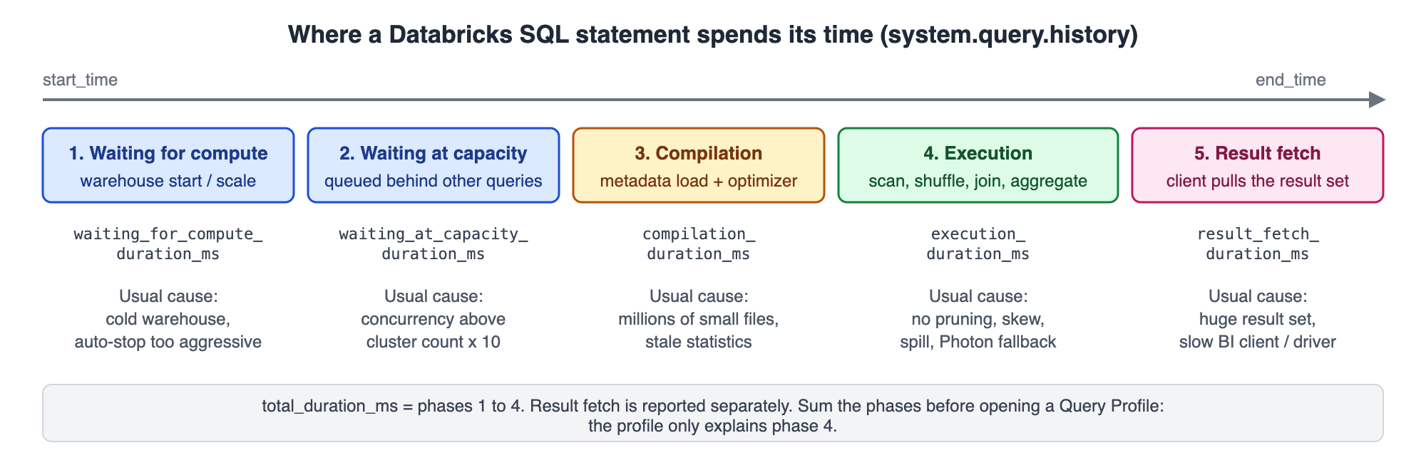
The query below ranks the slowest statements from the last 24 hours and shows, for each, which phase owns the time. Access to this table is admin-only by default; grant a view over it to the engineering team rather than the raw table, because statement_text is redacted for anyone outside the databricks_pii_access group.
SELECT
    statement_id,
    executed_by,
    compute.type                                     AS compute_type,
    compute.warehouse_id,
    client_application,
    total_duration_ms / 1000.0                       AS total_s,
    waiting_for_compute_duration_ms / 1000.0         AS wait_compute_s,
    waiting_at_capacity_duration_ms / 1000.0         AS wait_queue_s,
    compilation_duration_ms / 1000.0                 AS compile_s,
    execution_duration_ms / 1000.0                   AS exec_s,
    result_fetch_duration_ms / 1000.0                AS fetch_s,
    read_files,
    pruned_files,
    ROUND(read_bytes / 1024 / 1024 / 1024, 2)        AS read_gib,
    ROUND(shuffle_read_bytes / 1024 / 1024 / 1024, 2) AS shuffle_gib,
    ROUND(spilled_local_bytes / 1024 / 1024 / 1024, 2) AS spill_gib,
    read_io_cache_percent,
    from_result_cache,
    LEFT(statement_text, 120)                        AS statement_head
FROM system.query.history
WHERE start_time >= CURRENT_TIMESTAMP() - INTERVAL 24 HOURS
  AND execution_status = 'FINISHED'
  AND statement_type = 'SELECT'
ORDER BY total_duration_ms DESC
LIMIT 50;
Read the row for the statement someone complained about and classify it. If wait_compute_s dominates, the warehouse was starting or adding a cluster. If wait_queue_s dominates, the statement sat behind other work. If compile_s is large relative to exec_s, the planner spent its time loading metadata. Only when exec_s owns the majority of the total does the Query Profile become the right tool. A large fetch_s with a large produced_rows is a client problem, not a warehouse problem, and no amount of warehouse sizing will change it.
Two columns deserve a note. from_result_cache = true means the result was served from cache, so the row tells you nothing about execution cost; look at cache_origin_statement_id for the run that actually did the work. And total_task_duration_ms, the sum of all task time across all cores, divided by execution_duration_ms gives an effective parallelism figure. A ratio near 1 on a Large warehouse means the query ran on essentially one core, which almost always points at skew (Step 4) or at a single-file table.
Step 2: Queueing and cold starts are warehouse problems, not query problems
Classic and Pro Databricks SQL warehouses admit roughly ten concurrent queries per cluster. Beyond that, statements queue and the row shows a non-zero waiting_at_capacity_duration_ms. Autoscaling reacts to estimated queue load rather than to the queue length itself: a statement that has waited five minutes triggers a scale-up, and the warehouse adds one to three clusters depending on the projected processing time. Scale-down happens only after fifteen consecutive minutes of low load. Databricks serverless warehouses replace this with Intelligent Workload Management, which predicts each incoming query's resource needs and provisions capacity when queue wait grows, but a queue is still a queue.
The system.compute.warehouse_events table records STARTING, RUNNING, SCALED_UP, SCALED_DOWN, STOPPING and STOPPED events with the resulting cluster_count. Joining it to query history shows whether the slow statement arrived at a cold or an undersized warehouse:
WITH slow AS (
    SELECT
        statement_id,
        compute.warehouse_id                      AS warehouse_id,
        start_time,
        waiting_for_compute_duration_ms,
        waiting_at_capacity_duration_ms,
        total_duration_ms
    FROM system.query.history
    WHERE start_time >= CURRENT_TIMESTAMP() - INTERVAL 7 DAYS
      AND (waiting_for_compute_duration_ms > 30000
           OR waiting_at_capacity_duration_ms > 30000)
),
last_event AS (
    SELECT
        s.statement_id,
        MAX_BY(e.event_type, e.event_time)       AS event_before_start,
        MAX_BY(e.cluster_count, e.event_time)    AS clusters_before_start,
        MAX(e.event_time)                        AS event_time
    FROM slow s
    JOIN system.compute.warehouse_events e
      ON e.warehouse_id = s.warehouse_id
     AND e.event_time <= s.start_time
    GROUP BY s.statement_id
)
SELECT
    s.warehouse_id,
    s.start_time,
    s.waiting_for_compute_duration_ms / 1000.0    AS wait_compute_s,
    s.waiting_at_capacity_duration_ms / 1000.0    AS wait_queue_s,
    s.total_duration_ms / 1000.0                  AS total_s,
    l.event_before_start,
    l.clusters_before_start,
    TIMESTAMPDIFF(SECOND, l.event_time, s.start_time) AS seconds_since_event
FROM slow s
JOIN last_event l USING (statement_id)
ORDER BY s.start_time;
Three patterns come out of this repeatedly. First, a warehouse with a ten-minute auto-stop that a scheduled dashboard hits every fifteen minutes pays the cold-start cost on every refresh; the fix is a longer auto-stop or a serverless warehouse, and it costs less than the wasted analyst time. Second, a warehouse pinned at one cluster serving forty BI users queues constantly; raising the maximum cluster count is the fix, not tuning the forty queries.
Third, and most common, nightly ETL and interactive analytics share one warehouse, so the analysts' queries queue behind a MERGE. Separate the write workload onto its own warehouse and the "slow query" tickets disappear without anyone touching the SQL.
Step 3: Compilation time and the small-file problem
In Databricks, compilation covers metadata loading and optimisation. On Delta tables the metadata is the transaction log, and the planner has to read enough of it to know which files exist and what their min/max statistics say. A table with three million small files after months of streaming inserts can push compilation past a minute even for a SELECT COUNT(*). A wide view stacked over a dozen such tables multiplies the effect.
Check the file count and average file size before assuming the optimizer is at fault:
DESCRIBE DETAIL sales.fact_orders;
-- Look at: numFiles, sizeInBytes, clusteringColumns, partitionColumns, minReaderVersion

SELECT
    numFiles,
    ROUND(sizeInBytes / 1024 / 1024 / 1024, 1)                 AS size_gib,
    ROUND(sizeInBytes / NULLIF(numFiles, 0) / 1024 / 1024, 1)  AS avg_file_mib
FROM (DESCRIBE DETAIL sales.fact_orders);
An average file size in the low single-digit megabytes on a multi-terabyte table is the diagnosis. OPTIMIZE compacts the files, and on Databricks Runtime 15.4 LTS and above the durable fix is liquid clustering, which replaces both Hive-style partitioning and ZORDER, supports up to four clustering keys, and reclusters incrementally on each OPTIMIZE. Converting an existing partitioned table is a metadata operation followed by a rewrite:
-- Databricks Runtime 15.4 LTS+ (Delta). Test on a clone first; the OPTIMIZE FULL rewrites the table.
CREATE TABLE sales.fact_orders_test SHALLOW CLONE sales.fact_orders;

ALTER TABLE sales.fact_orders_test
    CLUSTER BY (order_date, customer_id);

OPTIMIZE sales.fact_orders_test FULL;

-- Verify: numFiles should drop sharply and clusteringColumns should list the keys.
DESCRIBE DETAIL sales.fact_orders_test;
For tables you do not want to hand-tune, CLUSTER BY AUTO lets the platform pick keys from observed query patterns, and predictive optimization schedules the OPTIMIZE runs on managed tables. Both are reasonable defaults for the long tail; we still pick keys by hand for the ten largest fact tables in any estate, because those are the ones the long-running queries touch.
Step 4: Reading the Query Profile for execution-bound statements
Once the phase breakdown says execution owns the time, open the Databricks Query Profile from the query history sidebar. It renders the operator DAG with per-operator time, rows, peak memory and, on scans, the fraction of data pruned. One limitation matters in practice: a statement served from the result cache shows "Query profile is not available", so change the LIMIT or add a trivial predicate to force a fresh run before profiling.
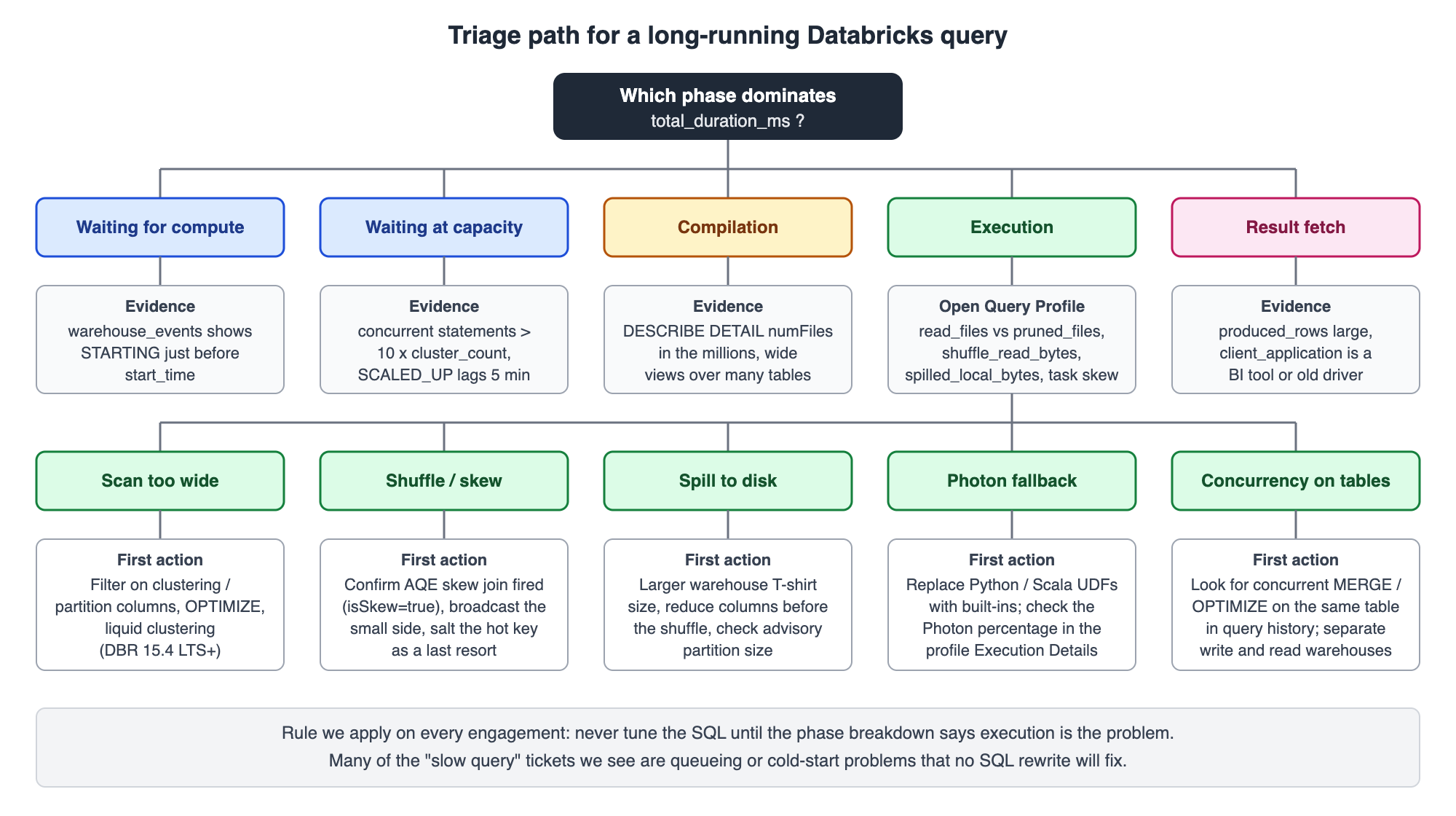
Four signals in the profile and in the history row account for most execution-bound Databricks long-running queries. The table below maps each signal to its usual cause and the evidence that confirms it.
| Signal | Where to read it | Usual cause | Confirming evidence |
|---|---|---|---|
| Scan reads most of the table | read_files vs pruned_files; scan operator pruning percentage |
Predicate not on clustering or partition columns; function wrapped around the filter column; statistics missing | pruned_files near zero while the WHERE clause is selective |
| Large shuffle, one slow task | shuffle_read_bytes; join operator max vs average task time |
Skewed join or aggregation key | total_task_duration_ms / execution_duration_ms far below core count |
| Spill to disk | spilled_local_bytes; operator "spill" metric |
Hash aggregate or sort larger than executor memory; too few shuffle partitions | Spill bytes comparable to shuffle_read_bytes |
| Low Photon share | Profile Execution Details: percentage of task time on Photon | Python or Scala UDF, unsupported expression, RDD or Dataset API | Spark UI shows blue (non-Photon) operators where orange is expected |
Scan too wide: predicates that cannot prune
Data skipping on Databricks Delta tables works on the min/max statistics of the first 32 columns by default, on the columns a table is clustered by, and on partition columns. A predicate such as WHERE DATE(order_ts) = '2026-09-01' defeats skipping because the statistics are on order_ts, not on DATE(order_ts). Rewrite it as a range on the raw column and the profile's scan operator will show the pruning percentage jump:
-- Before: function on the clustered column, no file skipping
SELECT customer_id, SUM(amount)
FROM sales.fact_orders
WHERE DATE(order_ts) = DATE '2026-09-01'
GROUP BY customer_id;

-- After: sargable range on the raw column, statistics prune files
SELECT customer_id, SUM(amount)
FROM sales.fact_orders
WHERE order_ts >= TIMESTAMP '2026-09-01 00:00:00'
  AND order_ts <  TIMESTAMP '2026-09-02 00:00:00'
GROUP BY customer_id;
Confirm the change with the same history query from Step 1: read_files should fall and pruned_files should rise for the new statement. If it does not, the column is probably not within the statistics set; check delta.dataSkippingStatsColumns in the table properties and set it explicitly for wide tables.
Shuffle skew: the single hot key
Skew is the failure mode that makes a 64-core Databricks warehouse behave like a 1-core one. A join on customer_id where one sentinel value such as -1 or 'UNKNOWN' owns 30% of the rows sends that 30% to a single shuffle partition, and the stage cannot finish until that one task does.
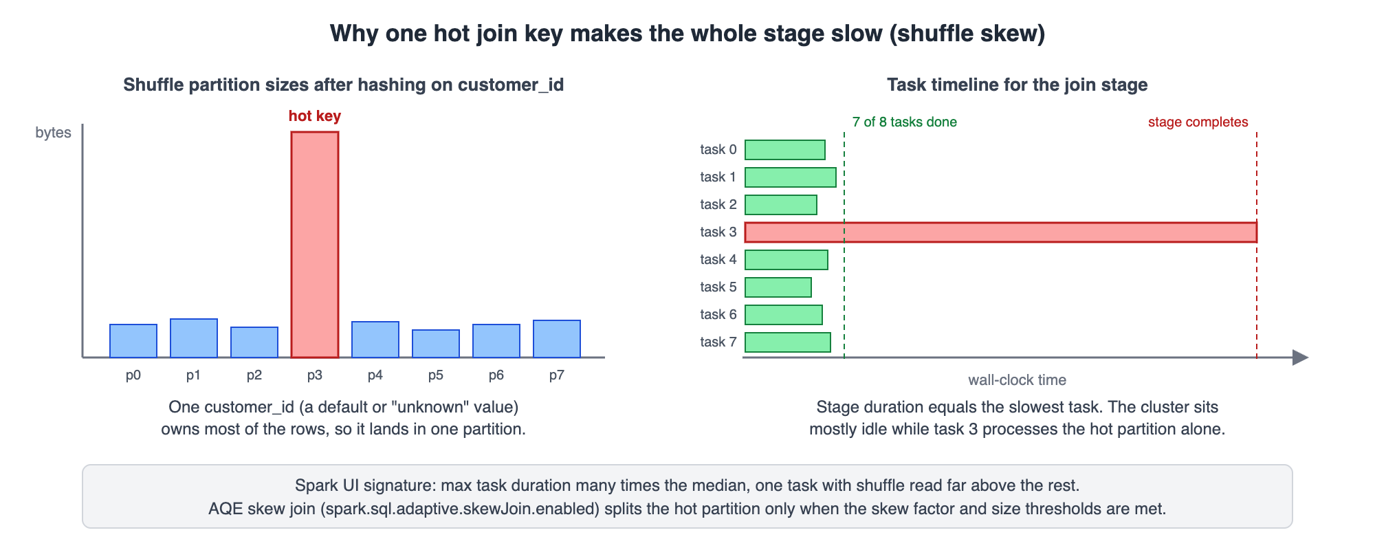
Adaptive Query Execution is on by default in Databricks (spark.databricks.optimizer.adaptive.enabled = true) and its skew-join handling (spark.sql.adaptive.skewJoin.enabled = true) splits a partition when it exceeds spark.sql.adaptive.skewJoin.skewedPartitionFactor (default 5) times the median and the size threshold. It only applies to sort-merge and shuffle-hash joins, and it cannot help a skewed GROUP BY. In the Spark UI the evidence is an AdaptiveSparkPlan node whose final plan shows SortMergeJoin with isSkew=true; if that flag is absent while the task histogram shows one straggler, AQE did not consider the partition skewed enough. From a notebook, the following prints the final plan with runtime statistics:
# PySpark, Databricks Runtime 15.4 LTS+ (AQE final plan is shown after an action)
df = (spark.table("sales.fact_orders").alias("o")
      .join(spark.table("sales.dim_customer").alias("c"), "customer_id")
      .groupBy("c.region").sum("o.amount"))

df.collect()
df.explain(mode="formatted")   # look for isFinalPlan=true and isSkew=true on the join node

# Quantify the skew directly before changing anything
(spark.table("sales.fact_orders")
      .groupBy("customer_id").count()
      .orderBy("count", ascending=False)
      .limit(10)
      .show())
The staged fix is: first, filter or coalesce the sentinel key before the join if the business logic allows it; second, broadcast the dimension if it fits under spark.databricks.adaptive.autoBroadcastJoinThreshold (30 MB by default; a BROADCAST hint raises it for one query); third, salt the hot key by appending a random suffix on the fact side and exploding the dimension side across the same suffix range. Salting is the last resort because it multiplies the dimension and complicates every downstream query, so keep it inside a view.
Spill: when the shuffle partition does not fit in memory
Non-zero spilled_local_bytes means a sort or hash aggregate wrote its working set to local disk. On Databricks SQL warehouses the lever is warehouse size, since memory per executor scales with the T-shirt size, and the honest question is whether the query needs the memory or wastes it. A SELECT * feeding a wide aggregate carries every column through the shuffle; projecting only the grouping and measure columns before the aggregate often removes the spill without any hardware change.
On jobs compute, spark.sql.adaptive.advisoryPartitionSizeInBytes (64 MB default) sets the target size AQE coalesces to; raising the number of shuffle partitions for a single heavy stage is a legitimate tactic when a small number of very large partitions spill.
Photon fallback
Photon is the default engine on Databricks SQL warehouses and on classic all-purpose and jobs compute. It covers scans, filters, projections, hash joins, hash aggregates and window functions on the common types, but it does not execute Python or Scala UDFs, RDD or Dataset API code, or stateful streaming. When it hits an unsupported expression it falls back to the JVM engine for that operator, correctly but slowly.
The profile's Execution Details panel reports the percentage of task time on Photon; anything well below 100% on a pure-SQL query deserves a look at the operator list. In the Spark UI for a cluster, Photon operators render in orange and JVM operators in blue, so the fallback boundary is visible at a glance. The fix is almost always to replace the UDF with a built-in, a higher-order function or a SQL expression:
# Python UDF: forces Photon fallback and per-row serialisation
from pyspark.sql.functions import udf, col, transform, upper
from pyspark.sql.types import ArrayType, StringType

@udf(returnType=ArrayType(StringType()))
def upper_tags(tags):
    return [t.upper() for t in tags] if tags else []

slow_df = spark.table("crm.accounts").withColumn("tags_u", upper_tags(col("tags")))

# Built-in higher-order function: stays inside Photon
fast_df = spark.table("crm.accounts").withColumn("tags_u", transform(col("tags"), lambda t: upper(t)))
Step 5: Long-running jobs and notebooks on classic compute
Databricks jobs and notebooks running on all-purpose or jobs compute do not appear in system.query.history unless they run on serverless compute or route through a warehouse. For those, the starting point is system.lakeflow.job_run_timeline and system.lakeflow.job_task_run_timeline, which carry one row per run per hour of runtime, so a task that ran for three hours appears as three rows sharing a run_id. The query below finds tasks whose latest run exceeded their 30-day median by a factor of two, which is the pattern behind most "the nightly job is late" escalations:
WITH task_runs AS (
    SELECT
        workspace_id,
        job_id,
        task_key,
        run_id,
        MIN(period_start_time)                                  AS started_at,
        MAX(period_end_time)                                    AS ended_at,
        TIMESTAMPDIFF(SECOND, MIN(period_start_time), MAX(period_end_time)) AS duration_s,
        MAX_BY(result_state, period_end_time)                   AS result_state
    FROM system.lakeflow.job_task_run_timeline
    WHERE period_start_time >= CURRENT_TIMESTAMP() - INTERVAL 30 DAYS
    GROUP BY workspace_id, job_id, task_key, run_id
),
baseline AS (
    SELECT
        job_id,
        task_key,
        PERCENTILE_APPROX(duration_s, 0.5)                      AS median_s,
        PERCENTILE_APPROX(duration_s, 0.95)                     AS p95_s
    FROM task_runs
    WHERE result_state = 'SUCCEEDED'
    GROUP BY job_id, task_key
),
latest AS (
    SELECT *
    FROM task_runs
    QUALIFY ROW_NUMBER() OVER (PARTITION BY job_id, task_key ORDER BY started_at DESC) = 1
)
SELECT
    j.name                                                      AS job_name,
    l.task_key,
    l.started_at,
    l.duration_s,
    b.median_s,
    b.p95_s,
    ROUND(l.duration_s / NULLIF(b.median_s, 0), 1)              AS slowdown_factor
FROM latest l
JOIN baseline b USING (job_id, task_key)
JOIN system.lakeflow.jobs j
  ON j.job_id = l.job_id
 AND j.workspace_id = l.workspace_id
 AND j.delete_time IS NULL
WHERE l.duration_s > 2 * b.median_s
ORDER BY slowdown_factor DESC;
With the task identified, the Spark UI for the run's cluster is the equivalent of the Query Profile. Open the SQL/DataFrame tab, find the longest query, and read its stages. The stage table shows task count, median and maximum task duration, shuffle read and spill per stage, and the same four causes from Step 4 apply. A stage with 200 tasks where the maximum duration is twenty times the median is skew. A stage with spill in the gigabytes is a memory-bound aggregate.
A stage whose input size is the whole table on a query with a selective predicate is a pruning failure, and dynamic file pruning (on by default since Databricks Runtime 10.4 LTS) only helps when the filtering table is joined, not when the predicate hides behind a function.
Two cluster-level checks are worth doing before any code change. Confirm that Photon is enabled on the Databricks cluster, since jobs created years ago often predate the default. And confirm that the cluster is not sharing a node pool with an interactive cluster that has auto-termination disabled, because "the job is slow" is sometimes "the job got half the nodes".
Step 6: Catch regressions before users report them
Troubleshooting long-running queries in Databricks after the fact is expensive. The same system tables support a regression check that runs as a scheduled Databricks SQL alert. The query below fingerprints statements by their first 200 characters, computes a rolling seven-day p95, and flags any fingerprint whose last-hour p95 exceeds the baseline by 50%. Tagging statements with query_tags from the client (supported on SQL warehouses) makes the grouping far more reliable than a text prefix, and we recommend that every BI tool and job set a tag identifying the report or pipeline.
WITH fingerprinted AS (
    SELECT
        COALESCE(query_tags['report'], SHA1(LEFT(statement_text, 200)))  AS fingerprint,
        start_time,
        total_duration_ms,
        spilled_local_bytes,
        waiting_at_capacity_duration_ms
    FROM system.query.history
    WHERE compute.type = 'WAREHOUSE'
      AND execution_status = 'FINISHED'
      AND from_result_cache = FALSE
      AND start_time >= CURRENT_TIMESTAMP() - INTERVAL 7 DAYS
),
baseline AS (
    SELECT
        fingerprint,
        PERCENTILE_APPROX(total_duration_ms, 0.95)  AS p95_baseline_ms,
        COUNT(*)                                    AS runs_7d
    FROM fingerprinted
    WHERE start_time < CURRENT_TIMESTAMP() - INTERVAL 1 HOUR
    GROUP BY fingerprint
    HAVING COUNT(*) >= 20
),
recent AS (
    SELECT
        fingerprint,
        PERCENTILE_APPROX(total_duration_ms, 0.95)  AS p95_recent_ms,
        SUM(spilled_local_bytes)                    AS spill_bytes_1h,
        MAX(waiting_at_capacity_duration_ms)        AS max_queue_ms_1h,
        COUNT(*)                                    AS runs_1h
    FROM fingerprinted
    WHERE start_time >= CURRENT_TIMESTAMP() - INTERVAL 1 HOUR
    GROUP BY fingerprint
)
SELECT
    r.fingerprint,
    r.runs_1h,
    b.runs_7d,
    ROUND(b.p95_baseline_ms / 1000.0, 1)            AS p95_baseline_s,
    ROUND(r.p95_recent_ms / 1000.0, 1)              AS p95_recent_s,
    ROUND(r.p95_recent_ms / b.p95_baseline_ms, 2)   AS regression_factor,
    ROUND(r.spill_bytes_1h / 1024 / 1024 / 1024, 2) AS spill_gib_1h,
    ROUND(r.max_queue_ms_1h / 1000.0, 1)            AS max_queue_s_1h
FROM recent r
JOIN baseline b USING (fingerprint)
WHERE r.p95_recent_ms > 1.5 * b.p95_baseline_ms
ORDER BY regression_factor DESC;
Three alert thresholds have earned their place in our Databricks runbooks: any statement with waiting_at_capacity_duration_ms above 60 seconds (warehouse undersized or shared with ETL), any warehouse whose hourly sum of spilled_local_bytes exceeds its hourly shuffle_read_bytes (memory-bound workload on the wrong size), and any table whose numFiles grows more than 20% week over week without a matching growth in sizeInBytes (small-file accumulation that will show up as compilation time within the month).
Version boundaries and what this method does not cover
The Databricks system tables described here require Unity Catalog and are populated for SQL warehouses and serverless compute; classic clusters appear only through the jobs timeline tables and the Spark UI. Liquid clustering is generally available for Delta on Databricks Runtime 15.4 LTS and above and for Apache Iceberg managed tables from 16.4 LTS in preview, with reads back to 13.3 LTS.
The AQE configuration names and defaults quoted above are the Databricks values, which differ from open-source Spark in the broadcast threshold and the spark.databricks prefix on the master switch. Databricks Runtime 18 LTS ships Apache Spark 4.1 and is the line we recommend for new jobs compute as of September 2026; verify feature availability against the runtime release notes before relying on any behaviour in a pinned older runtime.
This method also does not diagnose Delta Live Tables or Lakeflow pipeline latency, streaming trigger backlog, or Unity Catalog permission checks that occasionally surface as compilation time on tables with thousands of grants. Those have their own telemetry and deserve their own write-ups.
Where MinervaDB fits
Our Databricks lakehouse engineering practice applies exactly this evidence discipline on customer estates: phase breakdown first, warehouse topology second, SQL last. It sits inside our broader data analytics platform engineering service line, and the same team supports Snowflake, BigQuery and ClickHouse when the right answer is a different engine.
As always, test every change described here on a clone or in a staging workspace before applying it to production, keep a tested restore path for any table you rewrite with OPTIMIZE FULL, and treat the numbers in your own system.query.history as the only benchmark that matters. The official reference for the columns used in this post is the Databricks query history system table documentation.